Unsupervised Representation Learning with Predictive Coding

TLDR; Here’s a vanilla implementation of unsupervised predictive coding in PyTorch.

Predictive coding is an influential neuroscientific theory for the brain’s objective function—given some context, predict your sensory input. It can be implemented using local, Hebbian-like weight updates, which only require pre- and post-synaptic activity, which may provide a more bio-realistic implementation for credit assignment compared to backpropagation (Bogacz, 2017). Conceptually, these systems can also operate completely in parallel—both neural activity updates and weight updates. Unsupervised predictive coding models are generative models, which means their goal is often to reconstruct the data they observe—a nice property because there’s no need for manually curated human supervised labels. Counter to the flow of traditional artificial neural networks, where data flows left-to-right, input-to-output, predictive coding models invert this, and data flows right-to-left, starting with the latent state. In fact, it might even be better to think of the graph as flowing vertically, top-to-bottom. The top-level latent state passes through a layer of weights and attempts to predict the activity of the neurons at the level below. The prediction is compared to the actual activity, which drives an error. This error signal is propagated back to the top-level representation so that it can be adjusted to better predict the activity at the layer below. The representation at the layer below is also nudged towards the predicted activity to minimize error. This core motif can be repeated to form deep generative models. But even if you’re already a pro at these concepts and the math behind generative models, implementing these ideas correctly and in a way that recycles all the handy gradient definitions in PyTorch isn’t trivial. Luckily Rafal Bogacz’s lab has open-sourced a solid starting point. In this post, we’re going to unpack an implementation of vanilla unsupervised predictive coding. The Github repo for this tutorial can be found here: https://github.com/ToddMorrill/PredictiveCoding.

Figure 1: (A) the predictive coding motif, making predictions explicit, and (B) the typical visual you see in predictive coding papers (adapted from Orchard and Sun, 2019).

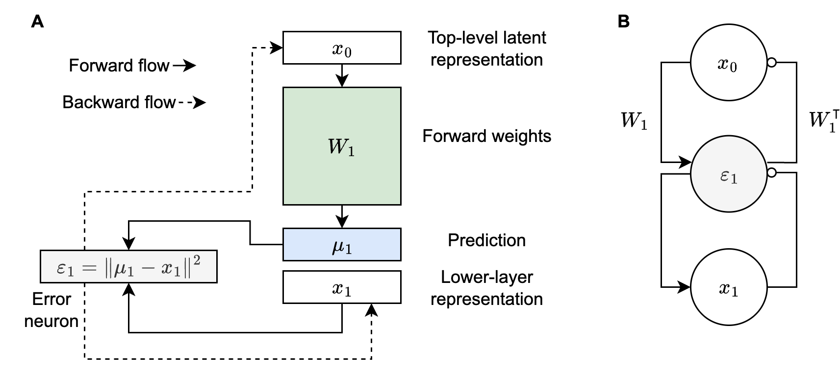
Figure 1A above is a graphical representation of what I described in the opening paragraph. Note that it makes explicit the role of top-down predictions, $\mu_1$, when evaluating error neurons. Another important point to note is that $\varepsilon_1$ nudges $x_1$ (and $x_0$) through its backward flow, so we’re never directly adjusting $\mu_1$—we’re adjusting $\mu_1$ through changes to $x_0$. Figure 1B is more typical of what you’ll see in predictive coding papers. I think this is because $\mu_1$ doesn’t really have an explicit analog in the proposed neural circuitry. In other words, neuroscientists may prefer to think about Figure 1B because it only shows value neurons (i.e., $x_0$ and $x_1$) and error neurons (i.e., $\varepsilon_1$), which is the hypothesized cortical circuitry, though evidence for explicit error neurons is mixed (Millidge et al., 2021). Nevertheless, Figure 1A is key to understanding the implementation below.

Implementing unsupervised predictive coding

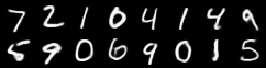
Our goal for this little experiment is to develop a “good” latent code in the sense that we can decode MNIST digits. In other words, given an MNIST digit, we’d like to determine if its latent code carries enough information for it to be correctly classified into one of the ten MNIST digit classes. You can either train a linear decoder or use $k$-nearest neighbors ($k$-NN) and then evaluate accuracy. Let’s start by highlighting some of the key parts of the code base, namely

• the model definition,
• the energy/loss functions,
• the optimizers,
• and the evaluation code.

Model definition

layers = [nn.Linear(input_size, hidden_size),
          activation_fn(), pc.PCLayer(),
          nn.Linear(hidden_size, hidden_size),
          activation_fn(), pc.PCLayer(),
          nn.Linear(hidden_size, output_size)]

This is a simple 3-layer feedforward neural network. The input is $x_0$ and has shape input_size, which is the size of the latent code. output_size is 784, which is the size of a flattened MNIST digit—our toy dataset for this little experiment. The pc.PCLayer() is the interesting bit. The input to a PCLayer is a $\mu$, or in other words a top-down prediction. To see this, note that the first two layers of the model above are nn.Linear(input_size, hidden_size) and activation_fn(), which means this produces $\mu_1$ in Figure 1A. The PCLayer() contains a parameter self._x (note that I’m referring to a PyTorch nn.Parameter() in the technical sense), which corresponds to $x_1$ in Figure 1A. This makes self._x persistent across model calls AND allows us to use PyTorch optimizers to nudge it (more on that below). Next, the definition of the PCLayer() has an argument energy_fn: typing.Callable = lambda inputs: 0.5 * (inputs['mu'] - inputs['x'])**2, which is what actually implements the error neuron, $\varepsilon_1$. We can sum over the vector size dimension to get a scalar loss value.

You might be asking yourself, where is $x_0$ implemented in all of this? It’s actually implemented in the PCTrainer class and is enabled through the use of PCTrainer.train_on_batch(is_optimize_inputs=True), which means the following will be defined: self.inputs = torch.nn.Parameter(self.inputs, True). So self.inputs will actually be our latent code, $x_0$, that we will use for evaluating our model using decoding accuracy (more on that below). Another question you might be wondering is, how do I know that gradients at the output layer won’t flow all the way back to the input layer, as they do with backpropagation? The answer follows from the way the compute graph has been defined. The self._x parameter defined on each PCLayer is a torch.nn.Parameter, which means it is a leaf node in the compute graph and therefore gradients stop at this point. The only connection between the earlier parts of the graph and the later parts of the graph is through the energy function. The higher layer is being supervised by the lower layer’s self._x through the energy function (and conversely $\mu_i$ is supervising $x_i$) but this is not the same as providing a direct backpropagation graph from the lower layer to the previous layer. So in summary, this shows how this predictive coding network is really just a chained collection of the motifs shown in Figure 1A and that all gradients flow to the self._x parameters and stop there.

Energy/loss functions

As noted above, each PCLayer in the network will have its own energy function. These can be summed together for the purpose of optimizing the neural activity and the weights of the network. However, we still haven’t specified how data enters into the picture and how to optimize the network with the input image clamped (this is the term folks use to describe part of the network being fixed at a particular value). In short, we’ll use a reconstruction loss by taking the output from the third and final linear layer—let’s call it $\mu_{3}$—and comparing it to the observed image using a squared-error loss. We specify PCTrainer.train_on_batch(loss_fn=loss_fn) and then define loss_fn as

def loss_fn(output, _target):
    return 0.5 * (output - _target).pow(2).sum()

which is basically the same type of loss as the layerwise energy functions, except now _target is actual observed data, whereas in the hidden layers self._x played the role of _target.

Optimizers

The PCTrainer takes four optimizer-related arguments as input: optimizer_x_fn, optimizer_x_kwargs, optimizer_p_fn, and optimizer_p_kwargs. The optimizer for the value neurons (the $x$ variables), optimizer_x_fn, isolates the self._x parameters in the model and targets updates on them, while optimizer_p_fn targets the weights of the model—the parameters of the nn.Linear layers. This enables a separation of timescales, where you first iterate the neural activity by calling the optimizer_x_fn until it reaches equilibrium (say 100-200 steps), at which point you can update the parameters with optimizer_p_fn. This can be thought of as perceptual inference (what am I looking at?) on a fast timescale and synaptic plasticity (improve my world model) at a slower timescale. This is also a current limitation of predictive coding—iterating your neural dynamics until you reach equilibrium is time-consuming and this is why future hardware that implements neurons directly into analog circuits would be valuable, because then you let physics implement the neural dynamics for you, which would enable far faster computation.

Evaluation

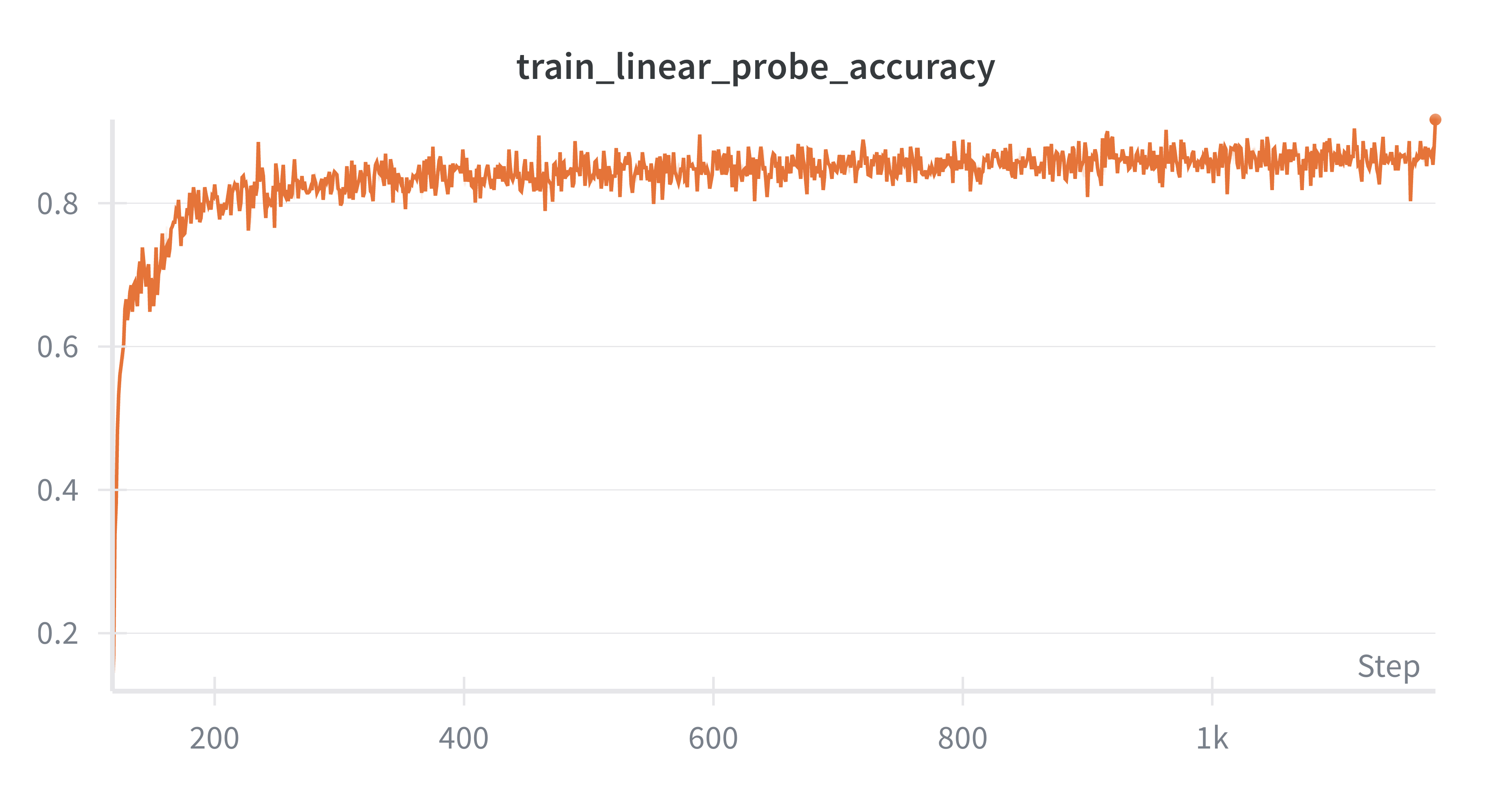
The layerwise energy functions and the final layer loss function provide natural measures to track during training. One would expect these to go down as the model learns. However, this doesn’t tell us how useful the model is. For that, we can train a linear probe model that takes latent representations ($x_0$s) from our primary predictive coding model and maps them to one of the ten MNIST digits. If we can do this accurately, it indicates that the representations may be learning something useful. If it can’t perform this task well (e.g., >98% accuracy is considered good), then it may indicate that we’re still missing something from our toolbox. The key evaluation code is in two places.

Linear probe accuracy. We train a linear probe alongside the predictive coding model (see train_linear_probe_batch in train.py). After training, we record the latent representations for all test set instances with the record_latent_representations function in train.py and then we use these representations to evaluate the learned representations using the linear probe model.

$k$-NN accuracy. We can also record latent representations of training set instances along with their associated labels and at test time, query these stored instances and use the labels of retrieved instances to create a non-parametric classifier. I’ve defined a KNNBuffer in utils.py to store these training set latent representations, while the evaluation code is defined as

def knn_classification(knn_buffer, representations, labels, k):
    """Perform kNN classification using the representations in the knn_buffer."""
    buffer_reps, buffer_labels = knn_buffer.get_all()
    # compute distances between representations and buffer_reps
    dists = torch.cdist(representations, buffer_reps)
    # get the indices of the k nearest neighbors
    knn_indices = torch.topk(dists, k, largest=False).indices
    # get the labels of the k nearest neighbors
    knn_labels = buffer_labels[knn_indices]
    # perform majority vote
    preds = []
    for i in range(knn_labels.size(0)):
        counts = torch.bincount(knn_labels[i])
        preds.append(torch.argmax(counts).item())
    preds = torch.tensor(preds).to(representations.device)
    # compute accuracy
    correct = (preds == labels).sum().item()
    acc = correct / labels.size(0)
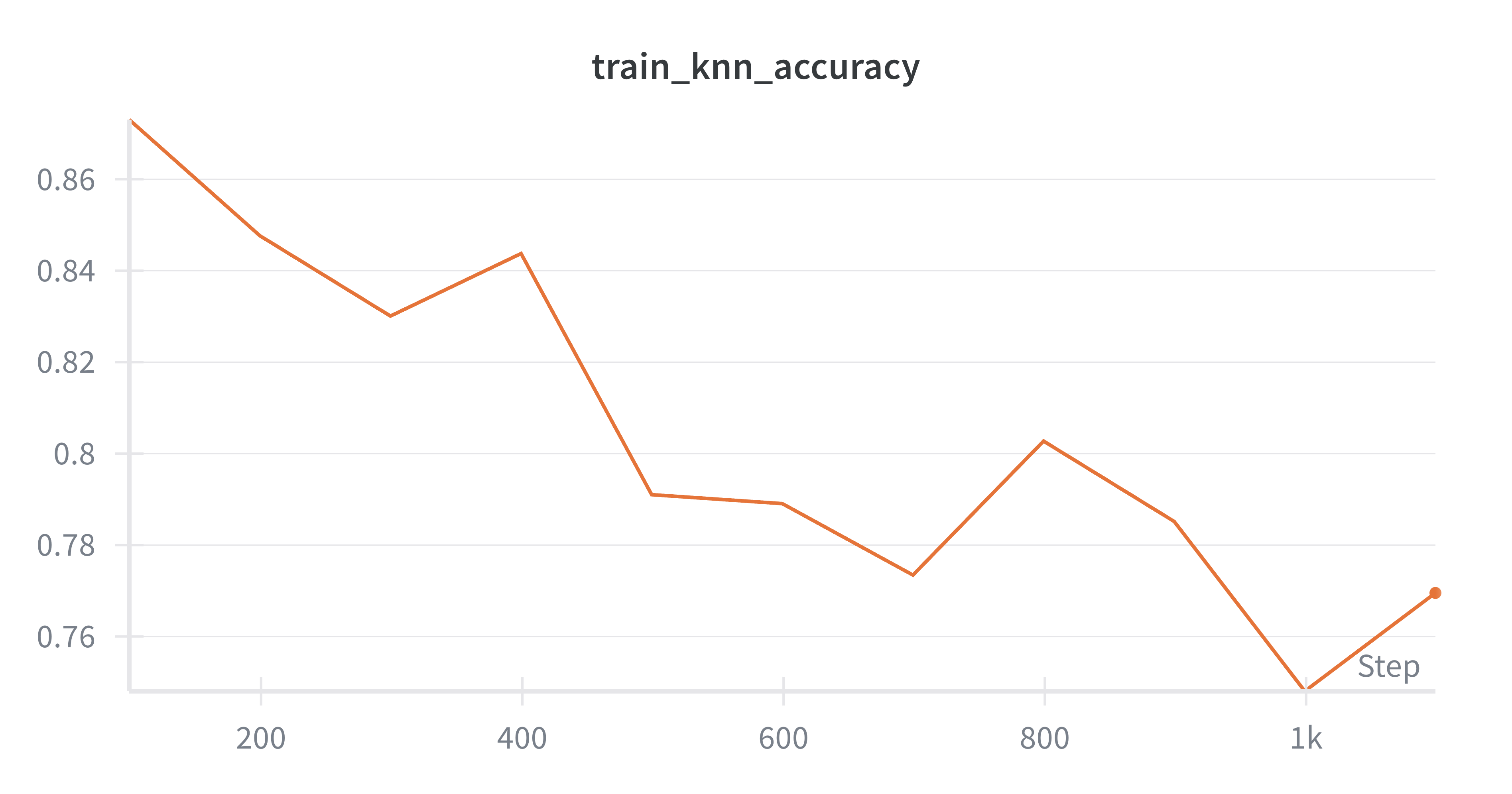
    return {'train_knn_accuracy': acc}

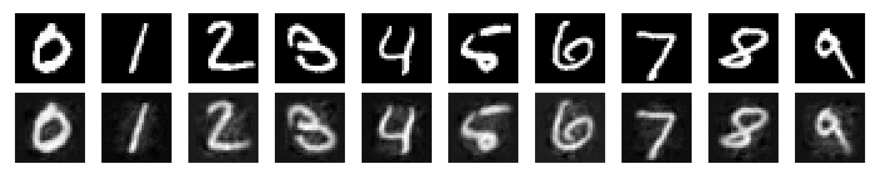
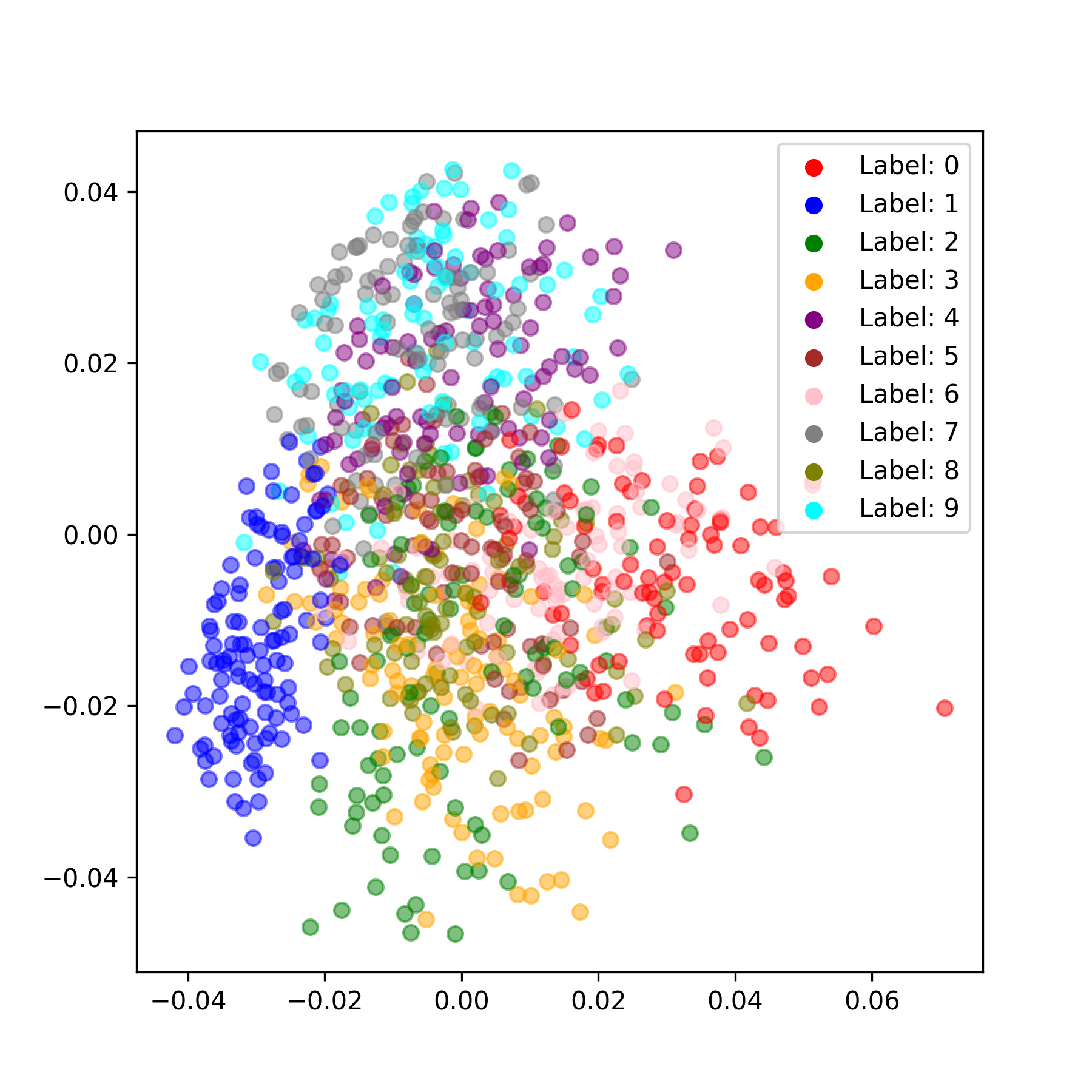
We can also generate some sample images and embed the latent representations using PCA, which provide a visual way to evaluate how well categorical structure emerges from the training process.

Figure 2: Sample generated MNIST digits. Top row shows originals, and bottom row shows generations.

Figure 3: PCA embedding of learned representations colored by MNIST digit. Clearly some class structure emerges.

Outro

Here are some observations I made while writing this up. I can achieve about 87% test set accuracy using the linear probe with basically zero hyperparameter tuning. The results are sensitive to the number of iterations you use for the neural dynamics (the time it takes for the neural activity to reach equilibrium) and in general, more iterations are better. This is a big pain point for predictive code and an active area of research (Pinchetti et al., 2024). This pipeline took about 10 minutes to run on my 4090 GPU, though I needed to use huge batch sizes to get any sort of sensible throughput (batch size 512). You could probably just increase the hidden dimensions (and maybe even just extend training) to improve decoding accuracy. $k$-NN accuracy starts high (in the high 80s) and gradually declines throughout training, which is a bit interesting and may be worth a closer look at what’s happening. I’m skipping the math for this tutorial but there are plenty of good resources out there giving motivation for predictive coding from a probabilistic modeling perspective (e.g., Bogacz, 2017). This project was vanilla unsupervised generative predictive coding. There are many worthy extensions, such as priors on neural activity—this model is very close to the Rao and Ballard 1999 model except I don’t place any sparsity priors on neural activity. You can also do supervised learning within this repo (Whittington and Bogacz, 2017). Overall, my sense is that there are still some major challenges to be overcome within predictive coding, but that it’s a worthy endeavor because it’s a way to investigate bio-inspired credit assignment (and may be a stepping stone to a training procedure for energy efficient spiking neural networks on next-generation hardware) and has some interesting properties in its own right, such as complete parallelism of the network.

Figure 4: Linear probe accuracy as training progresses.

Figure 5: k-NN accuracy as training progresses.