MS in Computer Science at Columbia: Semester Two, Spring 2023

TLDR; I finished the second semester (spring ‘23) of my MSCS program at Columbia.

Psetting.

I’m finally getting around to writing a recap of my second semester at Columbia. Similar to my first semester post, I’ll be going over the courses I took, the research I did, and the things I learned.

Summary

• took 2 classes: Advanced Algorithms (COMS 4232, Spring ‘23) with Professor Alex Andoni, High Performance Machine Learning (COMS 6998, Spring ‘23)
• continued working with Professor Kathleen McKeown as an NLP researcher on a DARPA project (2 courses worth of research credit $\implies$ full-credit load)
• started my foray into neuro-inspired computing with a focus on hyperdimensional computing

Coursework

I found two classes to be the sweet spot for maximizing learning while still being able to devote a decent amount of time (e.g., 15+ hours weekly) to research and exploration.

Advanced Algorithms

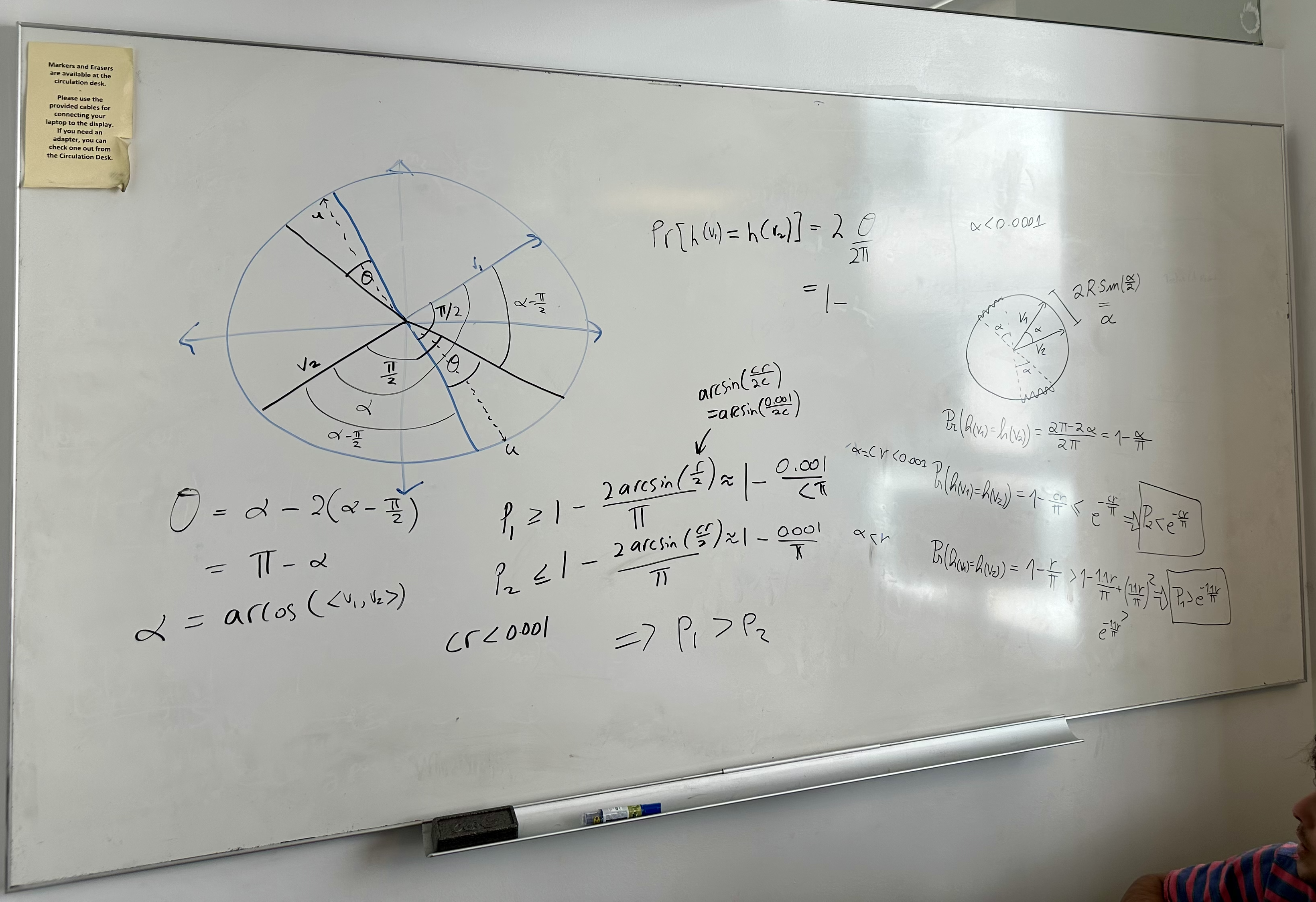
Advanced Algorithms was taught by Professor Alex Andoni. The course was approximately as difficult as a standard algorithms course but the big difference was that the focus was on approximation algorithms. This meant that we were often asked to come up with a solution to a problem that was not optimal but was within some factor of the optimal solution. Here’s a nice example that we covered early on in the class to illustrate the concept. Suppose your goal is to count the number of times a particular IP address visits your website, with the hopes of preventing a denial-of-service attack or something like that. Since we might have to record a lot of IP address’s, we want to save space on our count variable. We can use an algorithm called Morris’s Algorithm to do this. The algorithm is as follows.

Morris’s Algorithm

1. Initialize a variable $X = 0$.
2. Each time an IP address visits the website: \(X = \begin{cases} X + 1, & \text{with probability } \frac{1}{2^{X}} \\ X, & \text{with probability } 1 - \frac{1}{2^{X}} \end{cases}\)
3. Return $\hat{n} = 2^{X} - 1$

Intuitively, this procedure is flipping a biased coin, whose probability of coming up heads is decreasing each time $X$ is incremented. On the first website visit, $X = 0$ so $\frac{1}{2^{X}} = \frac{1}{2^{0}} = 1$, which means our estimate after the first visit is $2^{X} - 1 = 2^{1} - 1 = 1$! On the second visit, $X = 1$ so with probability $\frac{1}{2^{X}} = \frac{1}{2^{1}} = \frac{1}{2}$ we will increment $X$ and with probability $\frac{1}{2}$, we will leave $X$ at 1. The focus of the class was on answering questions like

1. Is this an unbiased estimator? (hint to the answer: yes - take the expectation of $\hat{n}$ and prove the result inductively)
2. What is the variance of this estimator? I.e., with high probability, how far off will our estimate be from the true value? (hint to the answer: we can use Chebychev bounds to show that this estimator concentrates reasonably well around the true value)
3. How many bits of space does this algorithm use (with high probability)? (hint to the answer: you can think of this procedure as storing the index for the power of 2 required to represent the count variable so instead of storing $\log(n)$ bits, which are needed to encode natural numbers in binary, we only need to store $\log(\log(n))$ bits. This can be shown using Markov’s inequality).

Notice that 2/3 of the questions above are probabilistic in nature due to the randomness of the procedure. This is one of those mind-blowing questions - does randomness confer some sort of algorithmic power? Other interesting topics included

1. hashing - solve the problem of constant time access to data records
2. sketching/streaming - Morris’ algorithm is an example of a streaming algorithm
3. nearest neighbor search - locality sensitive hashing is a technique that builds on the idea that similar points in your input space should hash to the same bucket
4. graph algorithms - max-flow algorithms (this felt the most like a standard algorithms course)
5. spectral graph theory - use the eigenvalues of the graph Laplacian to determine properties of the graph (e.g., number of connected components, etc.)
6. linear programming - use linear programming to solve problems like max-flow

This class had reasonable problem sets (typically only 3 problems per problem set), a midterm exam (no final), and a class research project. Our group summarized a line of work called Consistent Hashing, which attempts to minimize the amount of data movement required when a server is added or removed from a distributed system. It’s manageable to get an A in this class, but it’s on the trickier side with respect to the math.

High Performance Machine Learning

High Performance Machine Learning (HPML) was taught by Parijat Dube and Kaoutar El Maghraoui, both adjunct professors at Columbia who also work for IBM research. The focus of this class was on measuring and optimizing large-scale deep learning systems. Here are a few examples of how the class helped me.

1. This class exposed me to the memory constraints of modern GPUs powering deep learning systems (e.g., large language models). This class helped me make sense of PyTorch’s FSDP approach to distributed model training, which I directly applied in my data science job when trying to assess how much hardware we needed to train a large language model.
2. Next, suppose you do convince your manager to let you rent hundreds of GPUs in the cloud. The next question will be, am I making efficient use of my resources? Where are the bottlenecks? For example, I found that network interconnect bandwidth between GPUs really mattered for large language models and this class challenged me think about how that bandwidth interacted with the algorithms in use (e.g., ring-AllReduce gradient descent).
3. Here’s another concrete example. The big idea behind FlashAttention is tiling. In problem set 4, we implemented and measured the performance improvement of using tiling in matrix multiplications in CUDA code. I was blown away that such a fundamental technique that we studied in this course could have such a big research impact.

Other topics covered in this class included:

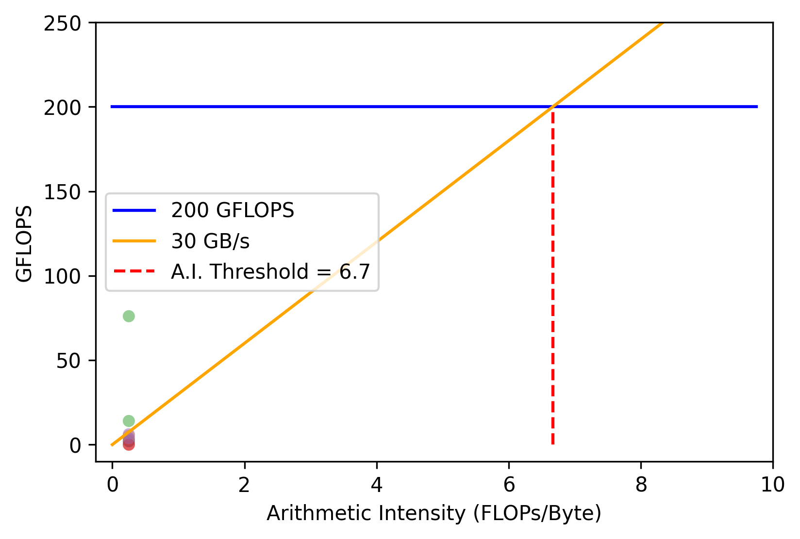
1. discussion of the key parameters affecting the performance of deep learning systems (e.g., GPU memory size and bandwidth, network interconnect bandwidth, FLOPS, etc.)
2. measurement techniques for assessing the performance of deep learning systems (e.g., profiling, benchmarking, roofline model, etc.)
3. a review of key deep learning ideas (e.g., optimizers and their memory footprints, etc.)
4. distributed deep learning (e.g., distributed gradient descent algorithms, data parallelism, model parallelism, etc.)
5. PyTorch internals (e.g., autograd, compiled computation graphs vs. dynamic computation, etc.)
6. CUDA programming
7. quantization, model pruning, and compression

Roofline diagram.

This class had 5 problem sets, quizzes every couple weeks, a final exam, and a class research project. Suffice it say that it was a hefty workload. Some of the problem sets were tricky (e.g., CUDA programming). The final exam wasn’t brutally challenging but many students felt like it was a lot to prepare for in the midst of finishing problem sets, quizzes, and a research project. My group measured the performance of a hyperdimensional computing (HDC) based natural language processing (NLP) model compared to a traditional transformer archictecture. I was excited about the HDC model because of its biological plausibility along with the nice properties that we showed (e.g., data efficiency, robustness to data corruption, etc.). You can read the report here. Overall, I really enjoyed the class and I think you can earn an A with an above average amount of effort.

Research

NLP

I continued working with Professor Kathleen McKeown as an NLP researcher on a DARPA project. I was hired under a little-known opportunity called the Advanced Masters Research (AMR) program. I wish this was better advertised and more opportunities like this were available at the master’s level. Some prominent researchers have written about the value of a research-oriented master’s degree, especially if you want to pursue a PhD but don’t have a ton of research experience. On top of the research experience I gained, my tuition was covered and I was paid a respectable stipend, in exchange for a fair amount of responsibility on the DARPA project.

The focus of the project is to apply NLP (translation, emotion detection, etc.) to analyze cross-cultural social interactions in real-time. These systems run on smartphones and extended reality glasses to assist business leaders, diplomats, and military members with negotiations, establishing partnerships, and planning. My responsibilities on the project were: 1) to develop systems that identify crucial points in social interactions that have the potential to improve or damage a relationship, and 2) lead Columbia’s integration effort, which involved shipping working software to DARPA that could be integrated with software developed by other research institutions.

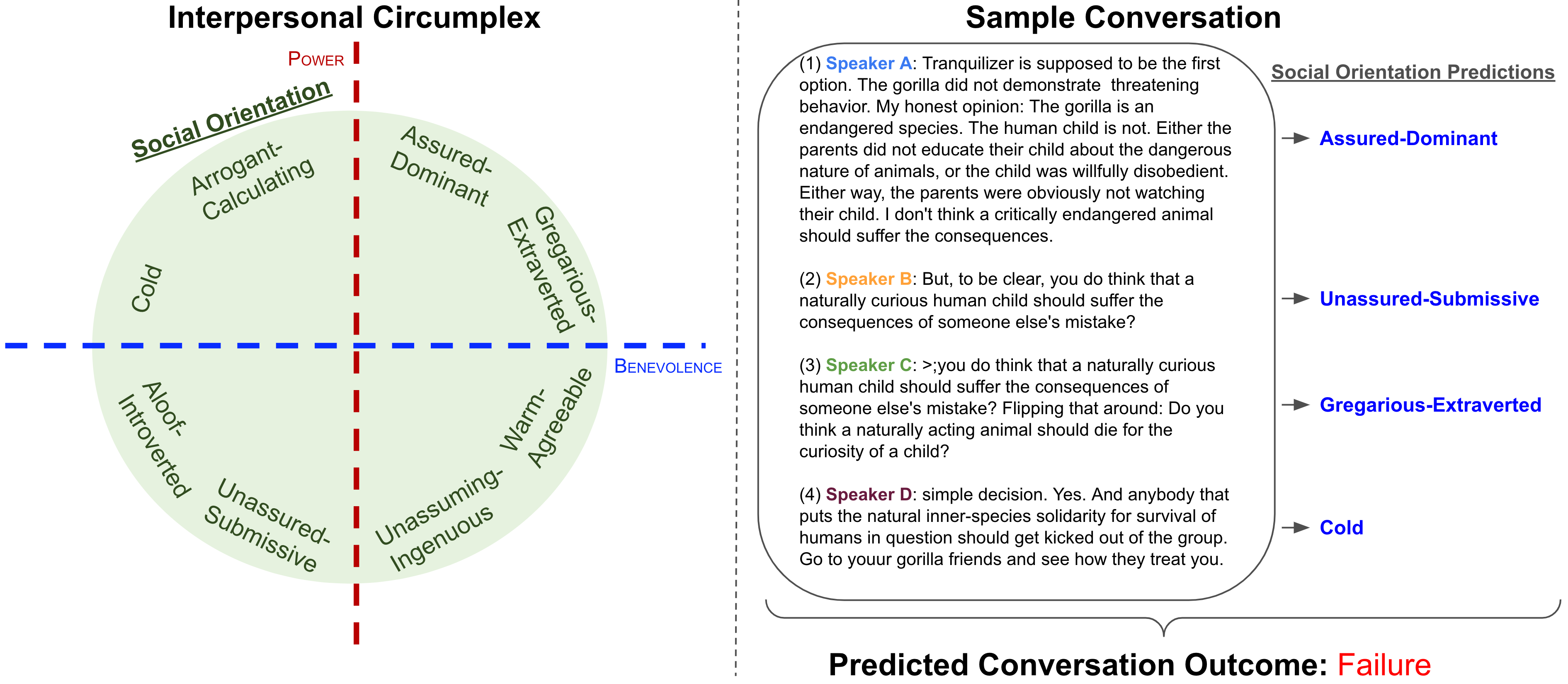
When I joined the project, I started working with a professor of social psychology to apply circumplex theory to the change point detection task (item 1) above). The research I pursued applied social orientation tags (e.g., Gregarious-Extraverted, Arrogant-Calculating, etc.) to conversation utterances and used circumplex theory to predict if a conversation was likely to succeed or fail. I later submitted this research to the LREC-COLING 2024 conference. As lead author on the paper, this was a particularly valuable learning experience, having to organize both advisors and peers to produce a scientifically sound and convincing paper while overcoming the setbacks that arose along the way.

Figure 1 from my circumplex paper.

Hyperdimensional Computing

In addition to the report that I wrote for the high performance machine learning class (linked above), which was more on the empirical side of things, I explored some of the theoretical aspects of HDC. In particular, I spent a good amount of time reading and deriving the results from a paper titled A Theoretical Perspective on Hyperdimensional Computing. Many of the results were robustness results showing that information encoded using HDC was increasingly resilient to random data corruption as the dimensionality of the representation grew. For instance, in Theorem 21 of the paper linked above, the authors show the robustness of a particular HDC encoding function to noise in the encoded space and defer a treatment of robustness to noise in the input space. I went on to show that the encoding function is robust to noise in the input space. This felt like an important distinction to make because you wouldn’t want a small change in, say, a single pixel of an image to cause a large change in the HDC representation of that image. This was a neat experience extending a result from a paper and I hope to continue exploring the theoretical aspects of HDC.