Yet Another Variational Autoencoders Tutorial

TLDR; I’m working through the details of VAEs once and for all.

Variational autoencoders (VAE) (Kingma & Welling, 2014) can feel a bit intimidating when you first encounter them. In principle, they’re just like regular autoencoders, right? 😅 Then you see there’s this weird KL divergence term, and all this reparametrization trick business and you’re like, “maybe I’m not tracking anymore.” In this post, I’m going to derive one particular - and arguably the most popular - instantiation of the VAE. There are so many good VAE tutorials out there but the ones that I came across are missing crucial details for an actual implementation. My hope is that this post is self-contained in the sense that we ask why or how at almost every opportunity and bottom out in all the gory mathematical details. This allows me to present a one-to-one correspondence between the math and PyTorch code so that you know why things are implemented the way that they are. The Github repo for this tutorial can be found here: https://github.com/ToddMorrill/vae.

Sample input MNIST digits.

Corresponding generated output MNIST digits.

This type of writing is influenced by so many people on the internet (e.g., Peter Bloem), who carefully take you through all the details. My thinking is that if you want to build or improve upon existing machine learning models then you need to really understand the math and the code. Also, this probably goes without saying, but I spent hours researching the material that went into this post, so don’t be put off if it takes you some time work through all the details presented here. This post assumes a pretty decent understanding of linear algebra, probability, and neural networks.

Preliminaries

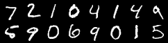
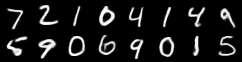
The VAE attempts to identify hidden (also called latent) low-dimensional structure in the world and use it to explain what we’re actually observing. What does this mean? Well, for instance, MNIST digits are images with $28\times 28 = 784$ pixels in the range $[0, 1] \subset \mathbb{R}$, where $0$ represents black and $1$ represents white. The question we can ask is, do we really need all $784$ pixels to represent the digit 2 (or 3, or 9, etc.) or can we actually use a much smaller dimensionality, such as 16? The VAE tells us that we can indeed compress the representation of the digit to very few dimensions and it also tells us how to do it.

We’re now going to define some notation. Since Lilian Weng does such a nice job, I’m going to adopt much of her notation and re-present many of her derivations here for completeness. In fact, you might find it useful to read her post before reading mine. My value-add will be to take this general formulation and present a specific implementation.

Symbol	Meaning
$\mathbf{X}$	The $d$ dimensional random variable representing the data.
$\mathbf{x}$	One realization of the data random variable.
$\mathbf{x}^{(i)}$	Each observed data point is a vector in $d$ dimensionts, $\mathbf{x}^{(i)} = [x^{(i)}_1, x^{(i)}_2, \dots, x^{(i)}_d]$
$\mathbf{x}’$	The reconstructed version of $\mathbf{x}$.
$\mathbf{Z}$	The low-dimensional random variable learned in the bottleneck layer (i.e., the latent low-dimensional structure).
$\mathbf{z}$	One realization of the latent random variable.
$\mathcal{D}$	The dataset, $\mathcal{D} = {\mathbf{x}^{(1)}, \ldots, \mathbf{x}^{(n)}}$, containing $n$ datapoints (i.e., $|\mathcal{D}| = n$).
$Q_{\phi}(\mathbf{Z}|\mathbf{X})$	Estimated posterior probability function, also known as a probabilistic encoder.
$P_{\theta}(\mathbf{X}|\mathbf{Z})$	Likelihood of generating the true data sample given the latent code, also known as the probabilistic decoder.

We are going to write down a joint distribution over our variables, $\mathbf{X}$ and $\mathbf{Z}$, factor this joint distribution according to the generative process (i.e., the process by which the data came about), and then start estimating our quantities of interest. The true joint distribution with real parameters $\theta^*$ factors as

\[\begin{align*} P_{\theta^*}(\mathbf{Z}, \mathbf{X}) &= P_{\theta^*}(\mathbf{Z})P_{\theta^*}(\mathbf{X} | \mathbf{Z}), \end{align*}\]

where the interpretation of this is that we can

1. Sample a $\mathbf{z}$ from the prior distribution $P_{\theta^*}(\mathbf{Z})$
2. Sample an $\mathbf{x}$ from the likelihood distribution $P_{\theta^*}(\mathbf{X} \mid \mathbf{Z}=\mathbf{z})$.

Since we don’t know $\theta^*$, we need to search for it. The maximum likelihood approach is to find the parameters $\theta$ that are most probable given the dataset, $P(\theta \mid \mathcal{D})$. By Bayes’ rule, we have

\[\begin{align*} P(\theta \mid \mathcal{D}) &= \frac{P(\mathcal{D} \mid \theta)P(\theta)}{P(\mathcal{D})}, \end{align*}\]

but we can ignore the denominator since it doesn’t depend on $\theta$. If this is the first time you’ve encountered this idea of disregarding the denominator, you can convince yourself that it’s OK to do this by noting that the denominator is a constant with respect to $\theta$. Suppose $P(\mathcal{D}) = 0.5$ for concreteness. Then, if we have two different $\theta$ values, such that $P(\theta_1|\mathcal{D}) > P(\theta_2|\mathcal{D})$, then we can multiply both sides by $0.5$ and we still have the inequality. In other words, scaling by a constant doesn’t change the relative ordering of which parameters are the best. Maximum likelihood estimation (MLE) makes another simplification by assuming that the prior $P(\theta)$ is uniform, which is equivalent to saying that all parameters are equally likely. So again, $P(\theta)$ is a constant and we can ignore it. This is where the name “maximum likelihood” comes from - we’re maximizing the likelihood of the data given the parameters - which is

\[\begin{align*} \arg\max_{\theta} P(\theta \mid \mathcal{D}) &= \arg\max_\theta P(\mathcal{D} \mid \theta)\\ &\equiv \arg\max_\theta P_{\theta}(\mathcal{D}) \tag{by definition of notation} \end{align*}\]

Expanding out $P_{\theta}(\mathcal{D})$, we have

\[\begin{align*} P_{\theta}(\mathcal{D}) &= \prod_{i=1}^n P_{\theta}(\mathbf{x}^{(i)}) \\ &= \prod_{i=1}^n \int P_{\theta}(\mathbf{x}^{(i)} \mid \mathbf{z})P_{\theta}(\mathbf{z})d\mathbf{z}. \end{align*}\]

One approach for finding the optimal parameters is to actually compute this integral, take the derivative of the expression with respect to $\theta$, set the derivative equal to zero, and solve for $\theta$. However, this is often intractable because the integral is high-dimensional. Here’s a nice example to illustrate that these types of integrals can be hard, even for seemingly trivial problems. If this feels hand-wavy, that’s because this is. I’m not really “proving” to you that this integral is hard for the case that we’ll be talking about this article, namely multivariate Gaussians. Maybe I’ll edit this post in the future and attempt this integral to really see why this is hard or impossible. This motivates the use of variational inference, which is a technique that introduces a surrogate distribution $Q_{\phi}(\mathbf{Z} \mid \mathbf{X})$ that we can work with more easily. The idea is to find the parameters $\phi$ that make $Q_{\phi}(\mathbf{Z} \mid \mathbf{X})$ as close as possible to the true posterior $P_{\theta}(\mathbf{Z} \mid \mathbf{X})$. At this point, you should be saying, wait, you said our objective was to maximize $P_{\theta}(\mathcal{D})$ but now you’re talking about $Q_{\phi}(\mathbf{Z} \mid \mathbf{X})$. Why? The answer is that we’re going to use $Q_{\phi}(\mathbf{Z} \mid \mathbf{X})$ to approximate $P_{\theta}(\mathbf{Z} \mid \mathbf{X})$ and then use this approximation to maximize $P_{\theta}(\mathcal{D})$. In order to build a little intuition for this, we can again appeal to Bayes’ rule to write

\[\begin{align*} P_{\theta}(\mathbf{Z} \mid \mathbf{X}) &= \frac{P_{\theta}(\mathbf{X} \mid \mathbf{Z})P_{\theta}(\mathbf{Z})}{P_{\theta}(\mathbf{X})}. \end{align*}\]

so in principle if we can approximate the lefthand side with $Q_{\phi}(\mathbf{Z} \mid \mathbf{X})$ and we know how to compute the numerator of the righthand side (this is the generative process), then we can compute the denominator of the righthand side. Since I’m being pedantic in this post, here’s what I’m saying mathematically.

\[\begin{align*} \overbrace{Q_{\phi}(\mathbf{Z} \mid \mathbf{X})}^{\text{computable approximation}} &\approx P_{\theta}(\mathbf{Z} \mid \mathbf{X}) = \frac{\overbrace{P_{\theta}(\mathbf{X} \mid \mathbf{Z})P_{\theta}(\mathbf{Z})}^{\text{computable}}}{\underbrace{P_{\theta}(\mathbf{X})}_{\text{want to estimate}}} \\ &\Rightarrow \\ P_{\theta}(\mathbf{X}) &\approx \frac{P_{\theta}(\mathbf{X} \mid \mathbf{Z})P_{\theta}(\mathbf{Z})}{Q_{\phi}(\mathbf{Z} \mid \mathbf{X})} \end{align*}\]

And we’re using $P_{\theta}(\mathcal{D})$ as our Monte Carlo approximation to $P_{\theta}(\mathbf{X})$ because that’s all we observe.

The VAE

We want the approximation $Q_{\phi}(\mathbf{Z} \mid \mathbf{X})$ to be as close as possible to $P_{\theta}(\mathbf{Z} \mid \mathbf{X})$. The natural next question is, how do we measure the distance between two distributions? The answer is the Kullback-Leibler (KL) divergence, which is a measure of how one probability distribution diverges from a second. The KL divergence is defined as

\[\begin{align*} D_{KL}(Q_{\phi}(\mathbf{Z} \parallel \mathbf{X})\|P_{\theta}(\mathbf{Z} \mid \mathbf{X})) &= \mathbb{E}_{Q_{\phi}(\mathbf{Z} \mid \mathbf{X})}\left[\log\frac{Q_{\phi}(\mathbf{Z} \mid \mathbf{X})}{P_{\theta}(\mathbf{Z} \mid \mathbf{X})}\right], \end{align*}\]

which we can expand as

\[\begin{align} D_{KL}(Q_{\phi}(\mathbf{Z} \parallel \mathbf{X})\|P_{\theta}(\mathbf{Z} \mid \mathbf{X})) &= \mathbb{E}_{Q_{\phi}(\mathbf{Z} \mid \mathbf{X})}\left[\log Q_{\phi}(\mathbf{Z} \mid \mathbf{X}) - \log P_{\theta}(\mathbf{Z} \mid \mathbf{X})\right] \\ &= \mathbb{E}_{Q_{\phi}(\mathbf{Z} \mid \mathbf{X})}\left[\log Q_{\phi}(\mathbf{Z} \mid \mathbf{X}) - \log \frac{P_{\theta}(\mathbf{X} \mid \mathbf{Z})P_{\theta}(\mathbf{Z})}{P_{\theta}(\mathbf{X})}\right] \tag{2}\\ &= \mathbb{E}_{Q_{\phi}(\mathbf{Z} \mid \mathbf{X})}\left[\log Q_{\phi}(\mathbf{Z} \mid \mathbf{X}) - \log P_{\theta}(\mathbf{X} \mid \mathbf{Z}) - \log P_{\theta}(\mathbf{Z}) + \log P_{\theta}(\mathbf{X})\right] \\ &= \mathbb{E}_{Q_{\phi}(\mathbf{Z} \mid \mathbf{X})}\left[\log Q_{\phi}(\mathbf{Z} \mid \mathbf{X}) - \log P_{\theta}(\mathbf{X} \mid \mathbf{Z}) - \log P_{\theta}(\mathbf{Z})\right] + \log P_{\theta}(\mathbf{X}) \tag{4}\\ &= \mathbb{E}_{Q_{\phi}(\mathbf{Z} \mid \mathbf{X})}\left[\log \frac{Q_{\phi}(\mathbf{Z} \mid \mathbf{X})}{P_{\theta}(\mathbf{Z})} - \log P_{\theta}(\mathbf{X} \mid \mathbf{Z})\right] + \log P_{\theta}(\mathbf{X}) \\ &= D_{KL}(Q_{\phi}(\mathbf{Z} \parallel \mathbf{X}) \mid P_{\theta}(\mathbf{Z})) - \mathbb{E}_{Q_{\phi}(\mathbf{Z} \mid \mathbf{X})}\left[\log P_{\theta}(\mathbf{X} \mid \mathbf{Z})\right] + \log P_{\theta}(\mathbf{X}) \tag{6}\\ \end{align}\]

where line 2 follows from Bayes’ rule, line 4 follows from the fact that

\[\mathbb{E}_{Q_{\phi}(\mathbf{Z} \mid \mathbf{X})} \left[\log P_{\theta}(\mathbf{X})\right] = \log P_{\theta}(\mathbf{X})\]

because $P_{\theta}(\mathbf{X})$ is a constant with respect to $\mathbf{Z}$, and line 6 follows from the definition of the KL divergence. Rearranging this last line, we have

\[\begin{align*} \log P_{\theta}(\mathbf{X}) - D_{KL}(Q_{\phi}(\mathbf{Z} \parallel \mathbf{X})\|P_{\theta}(\mathbf{Z} \mid \mathbf{X})) &= \underbrace{\mathbb{E}_{Q_{\phi}(\mathbf{Z} \mid \mathbf{X})}\left[\log P_{\theta}(\mathbf{X} \mid \mathbf{Z})\right]}_{\text{Reconstruction loss}} - \underbrace{D_{KL}(Q_{\phi}(\mathbf{Z} \parallel \mathbf{X}) \mid P_{\theta}(\mathbf{Z}))}_{\text{KL regularizer}} \\ &\equiv \text{Evidence Lower Bound (ELBO)} \end{align*}\]

and you can see that now we’re getting somewhere. The left-hand side contains the log-likelihood of the data, which is what we want to maximize. Also, maximizing the negative KL divergence is equivalent to minimizing the KL divergence because the KL divergence is always non-negative. Looking at the right-hand side, we have two terms that we should in principle be able to compute. The terms on the right-hand side also have nice interpretations. The first term is called the reconstruction loss and it measures how well the model is able to reconstruct the input data given the latent code $\mathbf{Z}$. The reconstruction loss is also known as the negative log-likelihood of the data under the model. The second term is called the KL regularizer and it encourages the approximate posterior $Q_{\phi}(\mathbf{Z} \mid \mathbf{X})$ to be close to the prior $P_{\theta}(\mathbf{Z})$.

This equation is also called the evidence lower bound (ELBO), which is a lower bound on the log-likelihood of the data. To see this, we have

\[\begin{align*} \log P_{\theta}(\mathbf{X}) - D_{KL}(Q_{\phi}(\mathbf{Z} \parallel \mathbf{X})\|P_{\theta}(\mathbf{Z} \mid \mathbf{X})) \leq \log P_{\theta}(\mathbf{X}), \end{align*}\]

which is true because the KL divergence is always non-negative (worth verifying). The ELBO is a lower bound on the log-likelihood of the data because the KL divergence is always non-negative. This is a good thing because it means that we can maximize the ELBO and we’re guaranteed to be improving the log-likelihood of the data.

The negation of the righthand side of the equation above is the loss function for the VAE

\[\begin{align*} \mathcal{L}_{VAE}(\theta, \phi) &= D_{KL}(Q_{\phi}(\mathbf{Z} \parallel \mathbf{X}) \mid P_{\theta}(\mathbf{Z})) - \mathbb{E}_{Q_{\phi}(\mathbf{Z} \mid \mathbf{X})}\left[\log P_{\theta}(\mathbf{X} \mid \mathbf{Z})\right] \end{align*}\]

and we optimize this function with respect to $\theta$ and $\phi$, which in practice tend to be parameters of a neural network. Since this post is exploring all the details, I just want to take a few more algebraic steps to link up this form of the ELBO with the form that you’ll see in other places (e.g., Wikipedia). Starting with our expression for the ELBO, we have

\[\begin{align*} \text{ELBO} &= \mathbb{E}_{Q_{\phi}(\mathbf{Z} \mid \mathbf{X})}\left[\log P_{\theta}(\mathbf{X} \mid \mathbf{Z})\right] - D_{KL}(Q_{\phi}(\mathbf{Z} \parallel \mathbf{X}) \mid P_{\theta}(\mathbf{Z})) \\ &= \mathbb{E}_{Q_{\phi}(\mathbf{Z} \mid \mathbf{X})}\left[\log P_{\theta}(\mathbf{X} \mid \mathbf{Z})\right] - \mathbb{E}_{Q_{\phi}(\mathbf{Z} \mid \mathbf{X})}\left[\log \frac{Q_{\phi}(\mathbf{Z} \mid \mathbf{X})}{P_{\theta}(\mathbf{Z})}\right] \\ &= \mathbb{E}_{Q_{\phi}(\mathbf{Z} \mid \mathbf{X})}\left[\log P_{\theta}(\mathbf{X} \mid \mathbf{Z})\right] - \mathbb{E}_{Q_{\phi}(\mathbf{Z} \mid \mathbf{X})}\left[\log Q_{\phi}(\mathbf{Z} \mid \mathbf{X})\right] + \mathbb{E}_{Q_{\phi}(\mathbf{Z} \mid \mathbf{X})}\left[\log P_{\theta}(\mathbf{Z})\right] \\ &= \mathbb{E}_{Q_{\phi}(\mathbf{Z} \mid \mathbf{X})}\left[\log \frac{P_{\theta}(\mathbf{X}, \mathbf{Z})}{Q_{\phi}(\mathbf{Z} \mid \mathbf{X})}\right]. \end{align*}\]

As a possibly useful aside, don’t be confused if you see other presentations of the VAE derive the ELBO by starting with the goal of maximizing the log-likelihood term, $\log P_{\theta}(\mathbf{X})$. The KL divergence, $D_{KL}(Q_{\phi}(\mathbf{Z} \parallel \mathbf{X})|P_{\theta}(\mathbf{Z} \mid \mathbf{X}))$, will fall out of algebraic manipulations of this approach and they’ll arrive at the same expression for the ELBO.

Instantiating the VAE

Many VAE tutorials stop here. But to get to an implementation we now need to start making some decisions about the functional form that these distributions will take. We’re going to assume that the prior $P_{\theta}(\mathbf{Z})$ is a multivariate Gaussian with mean $\mathbf{0}$ and covariance $\mathbf{I}$, which is the identity matrix.

We have a choice to make about the form of the likelihood function. One option in the case of MNIST digits is to assume that the likelihood $P_{\theta}(\mathbf{X} \mid \mathbf{Z})$ is a product of Bernoulli random variables, where the interpretation is that each pixel is a binary random variable (i.e., black or white). Another choice we could make is to model the likelihood as a multivariate Gaussian. In this case, we assume that the likelihood $P_{\theta}(\mathbf{X} \mid \mathbf{Z})$ is a multivariate Gaussian with mean \(\boldsymbol{\mu}_{\theta}\) and covariance matrix $\mathbf{I}$. We will later see how these choices get translated into concrete reconstruction loss functions.

We also can choose what functional form the approximate posterior $Q_{\phi}(\mathbf{Z} \mid \mathbf{X})$ will take. We’re going to assume that the approximate posterior is a multivariate Gaussian with mean \(\boldsymbol{\mu}_{\phi}\) and covariance \(\Sigma_{\phi}\), where $\Sigma_{\phi}$ is a diagonal matrix. This is a strong assumption because it assumes independent dimensions (i.e., no covariance structure) but it’s a common one, where the upsides are low computational complexity and more interpretable latent dimensions (each dimension is only coding for one thing).

The Reconstruction Loss

We’ll tackle the reconstruction loss first and then move on to the KL regularizer in the next section.

Case 1: Bernoulli Likelihood

Let’s assume that the likelihood $P_{\theta}(\mathbf{X} \mid \mathbf{Z})$ is a product of Bernoulli distributions. Concretely, this means that we’re going to take the logits of the output of the decoder and pass them through a sigmoid function to get the probabilities of the pixels being black or white. When I went to implement the VAE, I had no idea how to actually compute $P_{\theta}(\mathbf{X} \mid \mathbf{Z})$. The important observation to make is that in practice $P_{\theta}(\mathbf{X} \mid \mathbf{Z}) = P_{\theta}(\mathbf{X} \mid \mathbf{X’})$, where $\mathbf{X’}$ is the reconstructed version of $\mathbf{X}$. This is because the decoder is a deterministic function of the latent code $\mathbf{Z}$. To be really pedantic about this, suppose that $\mathbf{Z} = \mathbf{z}$ (i.e., some concrete value), and as a result the decoder outputs $\mathbf{X’} = \mathbf{x’}$. Then, the likelihood of generating the true data sample given the latent code is

\[\begin{align} P_{\theta}(\mathbf{X} \mid \mathbf{Z} = \mathbf{z}) &= \int_{\mathbf{x}'} P_{\theta}(\mathbf{X} \mid \mathbf{X'}=\mathbf{x}', \mathbf{Z}=\mathbf{z})P_{\theta}(\mathbf{X'}=\mathbf{x}' \mid \mathbf{Z}=\mathbf{z})d\mathbf{x}' \tag{7}\\ &= P_{\theta}(\mathbf{X} \mid \mathbf{X'} = \mathbf{x'}) \tag{8} \end{align}\]

where line 7 follows from conditioning on $\mathbf{X}’$ and then marginalizing out. Line 8 follows from a few observations. There’s only one value of $\mathbf{X’}$ that the decoder outputs given $\mathbf{Z}=\mathbf{z}$, which means that if you know $\mathbf{z}$, you know $\mathbf{x’}$. It also means that once you know $\mathbf{x’}$, the value of $\mathbf{z}$ no longer tells you anything new about $\mathbf{X}$. Mathematically, $\mathbf{X}$ is conditionally independent of $\mathbf{Z}$ given $\mathbf{X’}$. This observation also means that $P_{\theta}(\mathbf{X’}=\mathbf{x’} \mid \mathbf{Z}=\mathbf{z})$ acts as a Dirac delta function, which means that the integral collapses to a single value, namely the output of the decoder. This is a nice observation because it means that we can compute the reconstruction loss by comparing the output of the decoder to the input data. The reconstruction loss is the negative log-likelihood of the data under the model, which is

\[\begin{align*} -\log P_{\theta}(\mathbf{X} \mid \mathbf{Z}) &= -\log P_{\theta}(\mathbf{X} \mid \mathbf{X'}) \\ &= -\log \prod_{i=1}^d y_i^{x_i}(1-y_i)^{1-x_i} \\ &= -\sum_{i=1}^d x_i\log y_i + (1-x_i)\log (1-y_i), \end{align*}\]

where $y_i$ is the probability of the $i^{th}$ pixel being white, and $x_i$ is the ground truth value of the $i^{th}$ pixel in the input data. So you can see this product will collapse to a single term for each pixel. For instance, if the ground truth value of the $i^{th}$ pixel is $x_i = 1$ (i.e., white), then the loss for that pixel is $-\log y_i$. If the ground truth value of the $i^{th}$ pixel is $x_i = 0$ (i.e., black), then the loss for that pixel is $-\log (1-y_i)$. This is the binary cross-entropy loss, which is a common loss function for binary classification problems. This objective will attempt to make the output of the decoder as close as possible to the input data.

There’s one more detail to consider here. Don’t forget that in the derivation above we had to take an expectation over $\mathbf{Z}$ given a particular $\mathbf{X} = \mathbf{x}$, i.e.,

\[\mathbb{E}_{Q_{\phi}(\mathbf{Z} \mid \mathbf{X})}\left[\log P_{\theta}(\mathbf{X} \mid \mathbf{Z})\right].\]

In practice, people don’t actually compute this integral. Instead they take a Monte Carlo approximation of this expectation by sampling from $Q_{\phi}(\mathbf{Z} \mid \mathbf{X})$ and then averaging the loss over these samples. As you sample more points, the Monte Carlo approximation will converge to the true expectation. In practice (and in the original VAE paper), most people only sample a single $\mathbf{z}$ per data point and then average the loss over all the examples in the minibatch (e.g., $\approx 100$ samples) and this is often good enough. However, you can indeed sample multiple $\mathbf{z}$’s per data point and average the loss over all these samples and you might get better results.

In code this looks like

reconstruction_loss = F.binary_cross_entropy(x_reconstructed, x, reduction='sum')

where x_reconstructed is the output of the decoder and x is the input data. The reduction='sum' argument tells PyTorch to sum the loss over all the pixels.

Case 2: Gaussian Likelihood

In this case, we assume that the likelihood $P_{\theta}(\mathbf{X} \mid \mathbf{Z})$ is a multivariate Gaussian with mean $\mathbf{X}’$ by a similar reasoning as above and covariance matrix $\Sigma = \mathbf{I}$. The corresponding Gaussian distribution is then

\[\begin{align*} P_{\theta}(\mathbf{X} \mid \mathbf{X}') &= (2\pi)^{-d/2}\text{det}(\Sigma)^{-1/2}\exp\left(-\frac{1}{2}(\mathbf{X} - \mathbf{X}')^T\Sigma^{-1}(\mathbf{X} - \mathbf{X}')\right) \\ &= (2\pi)^{-d/2}\exp\left(-\frac{1}{2}\sum_{i=1}^d (x_i - x_i')^2\right), \end{align*}\]

Then if we take the log and negate (we want to minimize the loss, not maximize the log-probability), we have

\[\begin{align*} -\log P_{\theta}(\mathbf{X} \mid \mathbf{X}') &\approx \frac{1}{2}\sum_{i=1}^d (x_i - x_i')^2, \end{align*}\]

which should look like the familiar squared error loss. It’s very satisfying when an intuitive quantity like the squared error falls out of a principled derivation like this. Note that I’ve ignored the term $(2\pi)^{-d/2}$ because this is an additive factor after taking the log and can’t be reduced because it’s not a function of $\theta$. The $\frac{1}{2}$ term can indeed affect the optimization procedure because it’s essentially acting as a scaling factor that weighs the relative importance of the reconstruction loss (i.e., accuracy) against the KL regularizer (i.e., the complexity of the model). Anecdotally, I found that if you exclude the $\frac{1}{2}$ term, the model is more strongly encouraged to reduce the reconstruction error, which in turn results in a more complex model, which in turn results in a higher KL divergence loss term. As an aside there was a discussion of this very point on a popular ML podcast, Machine Learning Street Talk, where Karl Friston says it’s unclear if we should use a scaling term to control the relative importance of accuracy and complexity or if they should really be on the same scale.

In code this looks like

reconstruction_loss = 0.5 * F.mse_loss(x_reconstructed, x, reduction='sum')

where x_reconstructed is the output of the decoder and x is the input data. The reduction='sum' argument tells PyTorch to sum the loss over all the pixels.

The KL Regularizer

This is going to be the trickiest part of the tutorial. Deriving the KL regularizer term that you see in actual PyTorch implementations is a bit of a pain. Essentially, what we’re going to do is compute the KL divergence between two multivariate Gaussian distributions. I had to search all over to get a complete proof of this final form; you won’t find this spelled out in many VAE tutorials, and even those that provide a hint to the approach mostly appeal to the Matrix Cookbook, which provides theorems, not proofs. We will derive the KL divergence between two multivariate Gaussian distributions in the general case and then apply that result to our specific case. Consider two $d$-dimensional multivariate Gaussian distributions, $P(\mathbf{X})$ and $Q(\mathbf{X})$, with means $\boldsymbol{\mu}_P$ and $\boldsymbol{\mu}_Q$ and covariance matrices $\Sigma_P$ and $\Sigma_Q$, respectively. The KL divergence between these two distributions is given by

\[\begin{align*} D_{KL}(P(\mathbf{X}) \parallel Q(\mathbf{X})) &= \mathbb{E}_{P(\mathbf{X})}\left[\log\frac{P(\mathbf{X})}{Q(\mathbf{X})}\right] \\ &= \mathbb{E}_{P(\mathbf{X})}\left[\log P(\mathbf{X}) - \log Q(\mathbf{X})\right] \\ &= \mathbb{E}_{P(\mathbf{X})}[\frac{-d}{2}\log(2\pi) - \frac{1}{2} \log(\text{det}(\Sigma_p)) - \frac{1}{2}(\mathbf{X} - \boldsymbol{\mu}_{P})^T \Sigma^{-1}_P (\mathbf{X} - \boldsymbol{\mu}_{P}) \\ &\quad + \frac{d}{2}\log(2\pi) + \frac{1}{2} \log(\text{det}(\Sigma_Q)) + \frac{1}{2}(\mathbf{X} - \boldsymbol{\mu}_{Q})^T \Sigma^{-1}_Q (\mathbf{X} - \boldsymbol{\mu}_{Q})] \\ &= \frac{1}{2}\log\frac{\text{det}(\Sigma_Q)}{\text{det}(\Sigma_P)} - \frac{1}{2}\mathbb{E}_{P(\mathbf{X})}\left[(\mathbf{X} - \boldsymbol{\mu}_{P})^T \Sigma^{-1}_P (\mathbf{X} - \boldsymbol{\mu}_{P})\right] + \frac{1}{2}\mathbb{E}_{P(\mathbf{X})}\left[(\mathbf{X} - \boldsymbol{\mu}_{Q})^T \Sigma^{-1}_Q (\mathbf{X} - \boldsymbol{\mu}_{Q})\right] \end{align*}\]

Now we start inspecting these terms to simplify further. Consider

\[(\mathbf{X} - \boldsymbol{\mu}_{P})^T \Sigma^{-1}_P (\mathbf{X} - \boldsymbol{\mu}_{P}),\]

which is a scalar and can thus be thought of as a square $1\times 1$ matrix, which means the trace operater is well defined, so we have that

\[(\mathbf{X} - \boldsymbol{\mu}_{P})^T \Sigma^{-1}_P (\mathbf{X} - \boldsymbol{\mu}_{P}) = \text{Tr}\{(\mathbf{X} - \boldsymbol{\mu}_{P})^T \Sigma^{-1}_P (\mathbf{X} - \boldsymbol{\mu}_{P})\}.\]

It turns out that the trace of a product of matrices is invariant under cyclic permutations, which means that

\[\text{Tr}\{\mathbf{A}\mathbf{B}\mathbf{C}\} = \text{Tr}\{\mathbf{B}\mathbf{C}\mathbf{A}\} = \text{Tr}\{\mathbf{C}\mathbf{A}\mathbf{B}\}.\]

Not leaving a detail out, we’re going to prove this property. This property follows from the following result.

\[\begin{align*} \text{Tr}\{\mathbf {A} \mathbf {B} \} = \sum _{i=1}^{m}\left(\mathbf {A} \mathbf {B} \right)_{ii}=\sum _{i=1}^{m}\sum _{j=1}^{n}a_{ij}b_{ji}=\sum _{j=1}^{n}\sum _{i=1}^{m}b_{ji}a_{ij}=\sum _{j=1}^{n}\left(\mathbf {B} \mathbf {A} \right)_{jj}=\text{Tr}\{\mathbf {B} \mathbf {A} \} \end{align*}\]

So now if we let $\mathbf{A} = (\mathbf{X} - \boldsymbol{\mu}_{P})^T \Sigma^{-1}_P$ and $\mathbf{B} = (\mathbf{X} - \boldsymbol{\mu}_{P})$, then we can substitute \(\text{Tr} \{ (\mathbf{X} - \boldsymbol{\mu}_{P})(\mathbf{X} - \boldsymbol{\mu}_{P})^T \Sigma^{-1}_P \}\) and we have

\[\begin{align*} \frac{1}{2}\mathbb{E}_{P(\mathbf{X})}\left[(\mathbf{X} - \boldsymbol{\mu}_{P})^T \Sigma^{-1}_P (\mathbf{X} - \boldsymbol{\mu}_{P})\right] &= \frac{1}{2}\mathbb{E}_{P(\mathbf{X})}\left[\text{Tr}\{(\mathbf{X} - \boldsymbol{\mu}_{P})(\mathbf{X} - \boldsymbol{\mu}_{P})^T \Sigma^{-1}_P\}\right] \\ &= \frac{1}{2}\text{Tr}\{\mathbb{E}_{P(\mathbf{X})}\left[(\mathbf{X} - \boldsymbol{\mu}_{P})(\mathbf{X} - \boldsymbol{\mu}_{P})^T\right]\Sigma^{-1}_P\} \\ &= \frac{1}{2}\text{Tr}\{\Sigma_P \Sigma^{-1}_P\} \\ &= \frac{1}{2}\text{Tr}\{\mathbf{I}\} \\ &= \frac{d}{2} \\ \end{align*}\]

where we’ve interchanged $\mathbb{E}$ and $\text{Tr}$ by linearity. What is the definition of a linear function? It’s a function that satisfies the property that $f(a\mathbf{X} + b\mathbf{Y}) = af(\mathbf{X}) + bf(\mathbf{Y})$. The expectation and trace operators are linear functions because they satisfy this property. We’ve also relied on the fact that

\[\mathbb{E}_{P(\mathbf{X})}\left[(\mathbf{X} - \boldsymbol{\mu}_{P})(\mathbf{X} - \boldsymbol{\mu}_{P})^T\right]\]

is the covariance matrix!

Next we attack the third term, $\frac{1}{2}\mathbb{E}_{P(\mathbf{X})}\left[(\mathbf{X} - \boldsymbol{\mu}_{Q})^T \Sigma^{-1}_Q (\mathbf{X} - \boldsymbol{\mu}_{Q})\right]$. To do this, we’ll use the following Lemma.

Lemma: Suppose that $\mathbf{Y} \in \mathbb{R}^d$ is a random vector with mean $\boldsymbol{\mu}$ and covariance matrix $\Sigma$. Then for any matrix $\mathbf{A}\in \mathbb{R}^{d\times d}$, we have,

\[\begin{align*} \mathbb{E}[\mathbf{Y}^T\mathbf{A}\mathbf{Y}] = \boldsymbol{\mu}^T\mathbf{A}\boldsymbol{\mu} + \text{Tr}(\mathbf{A}\Sigma). \end{align*}\]

Proof: We have that

\[\begin{align*} \mathbf{Y}^T\mathbf{A}\mathbf{Y} &= [\boldsymbol{\mu} + (\mathbf{Y} - \boldsymbol{\mu})]^T\mathbf{A}[\boldsymbol{\mu} + (\mathbf{Y} - \boldsymbol{\mu})] \\ &= \boldsymbol{\mu}^T\mathbf{A}\boldsymbol{\mu} + \boldsymbol{\mu}^T\mathbf{A}(\mathbf{Y} - \boldsymbol{\mu}) + (\mathbf{Y} - \boldsymbol{\mu})^T\mathbf{A}\boldsymbol{\mu} + (\mathbf{Y} - \boldsymbol{\mu})^T\mathbf{A}(\mathbf{Y} - \boldsymbol{\mu}). \end{align*}\]

Taking expectations of both sides, we have that the middle two terms are 0 because $\mathbb{E}[\mathbf{Y} - \boldsymbol{\mu}] = 0$, yielding

\[\begin{align*} \mathbb{E}[\mathbf{Y}^T\mathbf{A}\mathbf{Y}] &= \boldsymbol{\mu}^T\mathbf{A}\boldsymbol{\mu} + \mathbb{E}[(\mathbf{Y} - \boldsymbol{\mu})^T\mathbf{A}(\mathbf{Y} - \boldsymbol{\mu})] \\ &= \boldsymbol{\mu}^T\mathbf{A}\boldsymbol{\mu} + \text{Tr}(\mathbf{A}\Sigma), \end{align*}\]

where we’ve repeated the trace trick that we performed above! $\blacksquare$

So now to apply this Lemma to our problem, we let $\mathbf{Y} = \mathbf{X} - \boldsymbol{\mu}_{Q}$ and $\mathbf{A} = \Sigma^{-1}_Q$. Note that this means $\mathbb{E}[\mathbf{Y}] = \mathbb{E}[\mathbf{X} - \boldsymbol{\mu}_{Q}] = \boldsymbol{\mu}_{P} - \boldsymbol{\mu}_{Q}$. This gives us

\[\begin{align*} \frac{1}{2}\mathbb{E}_{P(\mathbf{X})}\left[(\mathbf{X} - \boldsymbol{\mu}_{Q})^T \Sigma^{-1}_Q (\mathbf{X} - \boldsymbol{\mu}_{Q})\right] &= \frac{1}{2}[(\boldsymbol{\mu}_P - \boldsymbol{\mu}_{Q})^T \Sigma^{-1}_Q (\boldsymbol{\mu}_P - \boldsymbol{\mu}_{Q}) + \text{Tr}(\Sigma^{-1}_Q\Sigma_P)] \\ \end{align*}\]

Note that we’re relying on the fact that covariance is not affected by additive shifts in a random variable (i.e., $\text{Cov}(\mathbf{X} - \boldsymbol{\mu}_{Q})) = \text{Cov}(\mathbf{X}) = \Sigma_P$).

We can now substitute these results back into the KL divergence to get

\[\begin{align*} D_{KL}(P(\mathbf{X}) \parallel Q(\mathbf{X})) &= \frac{1}{2}\left[\log\frac{\text{det}(\Sigma_Q)}{\text{det}(\Sigma_P)} - d + (\boldsymbol{\mu}_P - \boldsymbol{\mu}_{Q})^T \Sigma^{-1}_Q (\boldsymbol{\mu}_P - \boldsymbol{\mu}_{Q}) + \text{Tr}(\Sigma^{-1}_Q\Sigma_P)\right]. \end{align*}\]

Returning back to our specific case, we assumed that the prior $P_{\theta}(\mathbf{Z})$ is a multivariate Gaussian with mean $\mathbf{0}$ and covariance $\mathbf{I}$, and we assumed that the approximate posterior $Q_{\phi}(\mathbf{Z} \mid \mathbf{X})$ is a multivariate Gaussian with mean $\boldsymbol{\mu}_{\phi}$ and covariance $\Sigma_{\phi}$ (reminder this is assumed to be diagonal). Concretely, $\boldsymbol{\mu}_{\phi}$ and $\Sigma_{\phi}$ are functions of the input $\mathbf{X}$ and produced by the encoder neural network. We can now substitute these into the KL divergence to get

\[\begin{align*} D_{KL}(Q_{\phi}(\mathbf{Z} \parallel \mathbf{X})\|P_{\theta}(\mathbf{Z})) &= \frac{1}{2}\left[\log\frac{\text{det}(\mathbf{I})}{\text{det}(\Sigma_{\phi})} - d + (\mathbf{0} - \boldsymbol{\mu}_{\phi})^T \mathbf{I}^{-1} (\mathbf{0} - \boldsymbol{\mu}_{\phi}) + \text{Tr}(\mathbf{I}^{-1}\Sigma_{\phi})\right] \\ &= \frac{1}{2}\left[-\log \text{det}(\Sigma_{\phi}) - d + \boldsymbol{\mu}_{\phi}^T \boldsymbol{\mu}_{\phi} + \text{Tr}(\Sigma_{\phi})\right]. \end{align*}\]

How do we implement this in PyTorch?

kl_divergence = 0.5 * torch.sum(-logvar - 1 + mu.pow(2) + logvar.exp())

Let’s unpack this slightly cryptic line of code. Assume that the neural network is producing the $\log$ of the variance instead of the variance directly and that logvar is a length-$d$ vector. The -1 will be broadcast over all $d$ dimensions, which corresponds to the $-d$ term in the equation above. The mu.pow(2) is the elementwise square of the mean $\boldsymbol{\mu}_{\phi}$, which corresponds to the $\boldsymbol{\mu}_{\phi}^T \boldsymbol{\mu}_{\phi}$ term in the equation above. The torch.sum function sums over all the elements of the vector $\boldsymbol{\mu}_{\phi} \odot \boldsymbol{\mu}_{\phi}$ (i.e., mu.pow(2)) to match the computation of that dot product. The logvar.exp() is elementwise exponentiation of the log-variance (this undoes the log operation), which corresponds to the $\text{Tr}(\Sigma_{\phi})$ term in the equation above.

And that’s how you derive the KL regularizer term in the VAE loss function!

Another Approach to the KL Regularizer

You can dispense with this detailed derivation and again take a Monte Carlo approximation of the KL divergence, which isn’t a bad approach as you can see here. However, in the VAE paper, the authors say that the closed form of the KL divergence is preferred because it provides lower variance estimates of the KL divergence term.

The Reparametrization Trick

This tutorial wouldn’t be complete without mentioning the reparametrization trick. The reparametrization trick is needed so that we can backpropagate through the sampling process for the approximate posterior $Q_{\phi}(\mathbf{Z} \mid \mathbf{X})$. Recall that the encoder is going to parameterize the approximate posterior as a multivariate Gaussian with mean $\boldsymbol{\mu}_{\phi}$ and covariance $\boldsymbol{\sigma}_{\phi}$. Suppose we sample a $\mathbf{z}$ from this distribution, which is easy enough to do. However, we can’t backpropagate through this sampling process because it’s not differentiable. Again, you should be asking why? So many tutorials just parrot this fact without explaining it. My intuition for this is that the gradient is attempting to capture how the output of a function changes with respect to its input. Suppose, we were to perturb one of the inputs to the sampling function, $\boldsymbol{\mu}_{\phi}$, just a little bit. The output of the sampling function might also correspondingly change just a little; after all the output is clearly related to the value of $\boldsymbol{\mu}_{\phi}$. BUT the output could nevertheless change wildly in an unpredictable way in response to a small change in $\boldsymbol{\mu}_{\phi}$. Clearly this isn’t what we want in a gradient. The reparametrization trick builds on this intution by pushing the randomness elsewhere so that we can indeed measure the gradient of the output with respect to the input. The reparametrization trick samples from a standard Gaussian and then transforms the samples to have the desired mean and covariance. In particular, we have

\[\begin{align*} \mathbf{Z} = \boldsymbol{\mu}_{\phi} + \boldsymbol{\epsilon} \odot \boldsymbol{\sigma}_{\phi}, \end{align*}\]

where $\boldsymbol{\epsilon} \sim \mathcal{N}(\boldsymbol{\epsilon}; \boldsymbol{0}, \mathbf{I})$ is a sample from a standard Gaussian, $\boldsymbol{\sigma}_{\phi}$ is the standard deviation corresponding to $\boldsymbol{\sigma}_{\phi}$, and $\odot$ is the elementwise product. To reiterate, since $\Sigma_{\phi}$ is a diagonal matrix, it is completely characterized by elements on the diagonal (i.e., a vector), which means we can just take the elementwise square root of the diagonal elements to get the standard deviation. If the covariance matrix wasn’t so “nice”, we would have to do a Cholesky decomposition to get the square root of the covariance matrix. While modeling the full covariance matrix might capture more rich structure in the data, it’s also more computationally expensive. Plus modeling the dimensions as independent may have the benefit of disentangling features. People like to try to control generations from the VAE by perturbing individual dimensions of the latent space with the implicit assumption that each dimension only controls one feature of the data (e.g., the thickness of the stroke in a digit).

So now the gradient of $\mathbf{Z}$ with respect to $\boldsymbol{\mu}_{\phi}$ and $\boldsymbol{\sigma}_{\phi}$ is well-defined, captures our intuition about small changes in the input and output, and we can backpropagate through the sampling process to adjust the parameters of the encoder. As always, we ask why is the correct equation? We can verify that this is indeed a sample from the desired distribution by taking the expectation and covariance. We have

\[\begin{align*} \mathbb{E}[\mathbf{Z}] &= \mathbb{E}[\boldsymbol{\mu}_{\phi} + \boldsymbol{\epsilon} \odot \boldsymbol{\sigma}_{\phi}] \\ &= \boldsymbol{\mu}_{\phi} + \mathbb{E}[\boldsymbol{\epsilon} \odot \boldsymbol{\sigma}_{\phi}] \\ &= \boldsymbol{\mu}_{\phi} + \boldsymbol{0} \odot \boldsymbol{\sigma}_{\phi} \\ &= \boldsymbol{\mu}_{\phi}, \end{align*}\]

and since each dimension of $\mathbf{Z}$ is independent of the others (i.e., has no covariance structure), we can analyze the covariance of $\mathbf{Z}$ by looking at its variance. We have

\[\begin{align*} \text{Var}[\mathbf{Z}] &= \text{Var}[\boldsymbol{\mu}_{\phi} + \boldsymbol{\epsilon} \odot \boldsymbol{\sigma}_{\phi}] \\ &= \text{Var}[\boldsymbol{\epsilon} \odot \boldsymbol{\sigma}_{\phi}] \\ &= \mathbb{E}[\boldsymbol{\epsilon}^2 \odot \boldsymbol{\sigma}_{\phi}^2] - \mathbb{E}[\boldsymbol{\epsilon} \odot \boldsymbol{\sigma}_{\phi}]^2 \\ &= \mathbb{E}[\boldsymbol{\epsilon}^2 \odot \boldsymbol{\sigma}_{\phi}^2] - \boldsymbol{0} \\ &= \mathbb{E}[\boldsymbol{\epsilon}^2]\odot \boldsymbol{\sigma}_{\phi}^2 \\ &= \text{Var}[\boldsymbol{\epsilon}]\odot \boldsymbol{\sigma}_{\phi}^2 \\ &= \boldsymbol{1}\odot \boldsymbol{\sigma}_{\phi}^2 \\ &= \boldsymbol{\sigma}_{\phi}^2\\ &= \boldsymbol{\Sigma}_{\phi}, \end{align*}\]

as desired. No magic here. This is a nice trick because it allows us to backpropagate through the sampling process.

In code this looks like

epsilon = torch.randn_like(mu)
z = mu + epsilon * sigma

where mu and sigma are the mean and standard deviation of the approximate posterior, respectively.

Conclusion

In this post we went through a detailed exploration of the VAE. We derived the loss function for the VAE, which is the negative ELBO, and we saw how to instantiate the VAE with concrete choices for the prior, likelihood, and approximate posterior. We also saw a one-to-one correspondence of these derivations in PyTorch code. I hope you enjoyed the post!

Bonus: Developing intuition about VAEs and the math behind the ELBO pays big dividends when you look at other topics like diffusion models and the free energy principle!