Detecting Entrained Signals - Part I

TLDR; I detected entrained brain waves from the EEG headset.

Continuing from the last post, I’ll recap what we’re working toward and the topic of this post. The goal for this experiment was to watch a video on a computer screen that flashes essentially a strobe light at a defined frequency such as 10 or 12hz and then be able to detect the entrained brainwaves in the EEG recording. If we can detect a signal in our brainwaves, we can use it to issue commands.

Here’s our outline:

1. Create the visual stimuli - previous post: Entrainment with Visual Stimuli
2. Record the EEG signal while watching the videos - today’s post
   • Video used for this analysis
   • Video that can be used for issuing commands
3. Analyze the data and try to detect the entrained signal - visual part of today’s post

Record the EEG signal while watching the videos

First, I’ll note that entrainment is not the most comfortable thing. You have to look at a blinking light and once the frequency gets above 10 hz it’s pretty trippy. It does seem to get better with time but generally, the goal is just to relax and watch the screen! Relax your thoughts and your gaze and soon you’ll be seeing patterns in the screen, which is a strong indication you’re entrained with the signal.

For this post, I’ll be analyzing the results of watching the 100 second long full screen video. When I created this video, I wanted to have 25 seconds of 8, 9, 10, and 11 hz respectively. Due to reasons explained in the previous post, I ended up with a video that has 50 seconds at 8.6hz, 25 seconds at 10hz, and 25 seconds at 12hz. This is fine, I just had to remind myself of that when I analyzed the results.

Analyze the data and try to detect the entrained signal

You can spot the entrained signals clear as day!

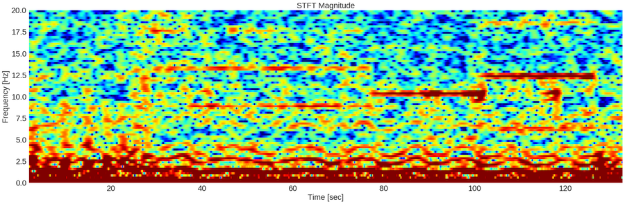
Since our ultimate goal is to be able to detect the signal of interest real time, I’ll focus on how we can generate this spectrogram and detect the signal using something called the Short Time Fourier Transform (STFT). I’ll explain some code below for illustration purposes. Once we understand the principles involved, we can move on to calculating the Fourier Transform for short time segments with more control.

nperseg=1024
noverlap=int(nperseg/1.05)
nfft=nperseg
plt.figure(figsize=(30,9))
# boundary=None got rid of the strips at the start and the end
# zero padding (nfft) interpolates and makes the spectrogram look smoother
# high noverlap gives you smooth temporal resolution
f, t, Zxx = signal.stft(raw_signal, sampling_rate, nperseg=nperseg, noverlap=noverlap, nfft=nfft, boundary=None)
plt.pcolormesh(t, f, 10*np.log10(np.abs(Zxx)),cmap=plt.get_cmap('jet'))
plt.title('STFT Magnitude', fontsize=22)
plt.ylabel('Frequency [Hz]', fontsize=22)
plt.xlabel('Time [sec]', fontsize=22)
plt.clim(-10, 5)
plt.ylim(0,20)
plt.xticks(fontsize=22)
plt.yticks(fontsize=22)
plt.show()

Let’s take it one line at time.

nperseg = 1024 is actually probably longer than necessary - it’s 4 seconds, given a sampling rate of 256hz. This is the length of the signal going into the Fourier Transform. Again, the Fourier Transform decomposes a signal into its component frequencies and their respective magnitudes. noverlap specifies the number of overlapping points. In other words, it becomes the step size. If your signal length is 1024 and your overlap is ~975, then your effective step size is ~49. 49samples/256samples/second is ~.2 of a second or 1/5th of one second. You can imagine your signal segment that is getting passed to the Fourier Transform as a tape reel. At each step, you update your tape reel with the 49 newest values (on the right side of the reel) and shift the older values to the left by 49. So that’s it! Each time you compute the STFT, you’re using a window in time that you define! Finally, the nfft parameter can be greater than or equal to the nperseg and it allows you to zero pad the segment. Ignoring zero padding is fine for now.

Let’s unpack what the signal.stft function returns. The first return value is f for frequencies. These are the component frequencies of your signal (e.g. 1hz, 2hz, 3hz, etc.). t is for time segments, which correspond to the time at which the FFT was taken (e.g. 0.2 seconds, 0.4 seconds, etc.). In our spectrogram above, we see a new column every ~0.2 seconds, corresponding to the step size of ~0.2 seconds. Finally, Zxx is an array of magnitudes of signals for each frequency for each timestep. Rows correspond to a specific frequency (refer to f to know which row indices correspond to which frequences), while columns correspond to a given timestep - it’s the same as you see in the spectogram! The spectrogram is colored based on the magnitude of the signal at different frequencies and timesteps.

Matplotlib can be tricky if you’re not super familiar with it. plt.colormesh gives you the spectrogram, while the 10*np.log10 of our signal gives the power decibels to scale the signal to a more reasonable range. I happen to like plt.get_cmap(‘jet’)) but you can experiment with other color maps. The only other thing worth noting (and isn’t self-explanatory) is plt.clim. I had to play around with these color ranges until I was pleased with the way the spectrogram looks.

So there it is! I think I’m going to stop here and continue explaining how to analyze this signal in the next post. In the next post, we’ll move beyond visual recognition of entrainment and move into a more rigorous algorithmic approach to signal detection.