KMeans Clustering Results
TLDR; KMeans can be used to discriminate between different time segments within an EEG recording.
Last time we left off with our motivation for exploring EEG data given that machine learning, and deep learning specifically, might do a better job identifying patterns in the EEG data. As a first exercise, I would like to accomplish two things: 1) do some exploratory data analysis on EEG data to better understand this data format, and 2) determine what features can be created and what they might be useful for. KMeans is a great algorithm for separating data into clusters when you don’t have labels. There are a number of assumptions to look out for and cluster evaluation is more of an art than a science but I’ll try to provide some color on this as we go through the results.
To recap, I recorded about a minute of 16 channel + accelerometer data. This data is a recording of sitting normally (eyes open), eyes closed (should see alpha waves), jaw clenching (lots of artifacts), and shaking my head side-to-side and front-to-back (see what the accelerometer picked up). My hypothesis is that KMeans might be able discriminate between the ~5 different actions above.
Preprocess the data
The data preprocessing steps can be overwhelming when first starting out with EEG data so let’s take it one step at a time and look at some code along the way. For the complete code, check out my script here.
signal_data = df['Channel_8']

# https://github.com/chipaudette/EEGHacker/blob/master/Data/2014-10-03%20V3%20Alpha/exploreData.py
# filter the data to remove DC
hp_cutoff_Hz = 1.0
print("highpass filtering at: " + str(hp_cutoff_Hz) + " Hz")
b, a = signal.butter(2, hp_cutoff_Hz/(sampling_rate / 2.0), 'highpass')  # define the filter
clean_signal = signal.lfilter(b, a, signal_data, 0) # apply along the zeroeth dimension

# notch filter the data to remove 60 Hz and 120 Hz interference
notch_freq_Hz = np.array([60.0, 120.0])  # these are the center frequencies
for freq_Hz in np.nditer(notch_freq_Hz):  # loop over each center freq
    bp_stop_Hz = freq_Hz + 3.0*np.array([-1, 1])  # set the stop band
    print("notch filtering: " + str(bp_stop_Hz[0]) + "-" + str(bp_stop_Hz[1]) + " Hz")
    b, a = signal.butter(3, bp_stop_Hz/(sampling_rate / 2.0), 'bandstop')  # create the filter
    clean_signal = signal.lfilter(b, a, clean_signal, 0)  # apply along the zeroeth dimension
One of the preprocessing steps requires bandpass filtering the raw EEG signals. There isn’t much to see below 1Hz in the brain and this range tends to contain a lot of noise so we’re going to filter that out. We’re also going to notch filter out 60Hz and its harmonic at 120Hz because 60Hz is the utility frequency used for electricity in the United States.
Once we’ve removed those frequency bands, we do a spectrogram plot to see what the recording looks like. A spectrogram plot is great because it conveys 3 pieces of information: 1) time along the x-axis, 2) frequency (Hz) along the y-axis, and 3) the magnitude of the signal from the color. What’s neat here is that it’s visually intuitive once you get familiar with it, and more interestingly, we can probably use these plots to conduct our deep learning experiments. For example, if you look at some of the speech-to-text deep learning architectures, you’ll see that they use spectrogram time slices that get fed to a convolutional recurrent neural network. In other words, a convolutional neural network runs over each fractional second spectrogram and the activation vector gets passed on to a recurrent neural network that translates speech-to-text. My team has worked with Baidu’s architecture so this experience should bootstrap some of our coding.
NFFT = int(sampling_rate*1) # length of the fft
overlap = NFFT - int(0.25 * sampling_rate)  # three quarter-second overlap

fig = plt.figure(figsize=(30, 9))

Pxx, freqs, bins, im = plt.specgram(clean_signal,NFFT=NFFT,\
                                    Fs=sampling_rate, noverlap=overlap, \
                                    cmap=plt.get_cmap('viridis'))

Pxx_perbin = Pxx * sampling_rate / float(NFFT)  #convert to "per bin"
# need to better understand that

# reduce size
# Pxx_perbin = Pxx_perbin[:, 1:-1:2]  # get every other time slice
# bins = bins[1:-1:2]  # get every other time slice

plt.pcolor(bins, freqs, 10*np.log10(Pxx_perbin), cmap=plt.get_cmap('viridis'))  # dB re: 1 uV
plt.clim(-15,15)
plt.xlim(bins[0], bins[-1])
plt.ylim(0,40)
plt.xlabel('Time (sec)',fontsize=22)
plt.ylabel('Frequency (Hz)',fontsize=22)
plt.xticks(fontsize=22)
plt.yticks(fontsize=22)
plt.show()
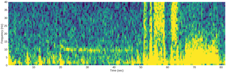
The above code plots a nice looking spectrogram of the ~83 second recording. In the first 20 seconds you can see what my normal state looks like followed by ~25 seconds of eyes closed. After that, you can see the artifacts associated with jaw clenching followed by head shaking side-to-side and front-to-back.
KMeans attempt 1
From here, we should just take a naïve pass at using the raw EEG signal plus the accelerometer data to see what KMeans comes up with using k=4 clusters.
scaler = preprocessing.StandardScaler()
training_data = scaler.fit_transform(df[data_cols])
cluster = KMeans(n_clusters=4)
results = cluster.fit_predict(training_data)
df['cluster_number'] = results

start_index = 0
duration=int(len(df.iloc[start_index:])/sampling_rate)
print("{} seconds of recording".format(duration))
df.iloc[start_index:]["cluster_number"].plot(figsize=(30,9))
plt.xlabel('Timestamp',fontsize=22)
plt.ylabel('Cluster Number',fontsize=22)
plt.xticks(fontsize=22)
plt.yticks(fontsize=22)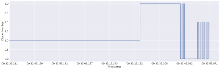
KMeans is probably heavily relying on signal magnitude to drive cluster assignment
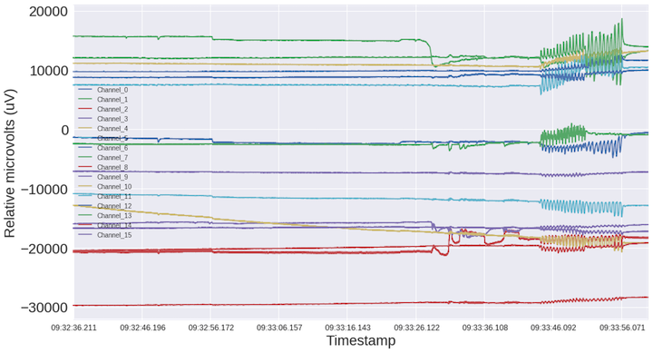
The above plot shows cluster assignment over time of each data point (1/256th of a second given a sampling rate of 256Hz). One neat observation here is that this first pass does a pretty good job breaking up the jaw clenching vs headshaking sections. It also appears to be making cluster assignments according to the back and forth movement of my head at the end of the recording. The only downside here is that it’s treating the whole first portion of the recording as one cluster and yet we know that there should an “eyes closed” cluster. What we need to do now is find the right feature to break this big first cluster up. Let’s move from the time domain to the frequency domain and summarize the frequency with the maximum magnitude, the mean frequency, the sum of the magnitude, and the power of the signal (i.e. mag**2) for a sliding window along the recording.
Before we move on, you may be wondering what preprocessing.StandardScaler() does. It is used to scale our features so that they have a mean of 0 and unit variance (variance of 1). This makes features with different scales comparable. KMeans is a (within cluster) variance minimization algorithm and if one of your dimensions is in dollars and one is yen, you’re likely to see clusters driven by yen just because there will appear to be more variance in that dimension. In our case, the raw EEG data and the accelerometer data have different scales so if we didn’t standardize the data, the raw signal would impact the final clustering results more than the accelerometer would.
Try generating a frequency summary for each timestep (timestep adjustable) for 1 channel of EEG Data (Channel 8/O2)
NB: I’m going to start with one channel for two reasons: 1) ease of initial analysis, and 2) if we create 4 features for each of the 16 channels, then we’ll have 64 features per timestep, which means we’ll need to start thinking about PCA due to the curse of dimensionality.
n = len(clean_signal) # length of the signal
k = np.arange(n) # array of timesteps in observations
T = n/float(sampling_rate) # number of sampling cycles
freqs = k/np.float(T) # two sides frequency range
freqs = freqs[range(n/2)] # one side frequency range # due to nyquist frequency

lower_freq = 0.
upper_freq = 40.
mask = np.logical_and(freqs >= lower_freq, freqs <= upper_freq)

Y = np.fft.fft(clean_signal)*2/n # fft computing and normalization # why normalize? again a result of the nyquist frequency
Y = Y[range(n/2)] # only taking half of the outputs
Y = np.abs(Y) # take the magnitude of the signals

# filter down to frequencies of interest
Y = Y[mask]
freqs = freqs[mask]

fig = plt.figure(figsize=(16, 9))
plt.plot(freqs, Y)
plt.xlabel("Frequency (hz)",fontsize=22)
plt.ylabel("Magnitude (uV)",fontsize=22)
plt.xticks(fontsize=22)
plt.yticks(fontsize=22)
plt.show()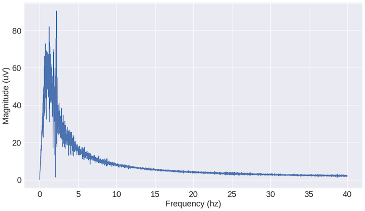
What we see above is a shift from the time domain to the frequency domain. Imagine the time domain as a bunch of sinusoid waveforms (because that’s what it is!) and what the frequency plot is doing is measuring the magnitude of the sinusoids at different oscillation frequencies. The result is a summary of the time domain signal. Instead of looking at the entire recording, we can look at smaller chunks of the recording and generate features that summarize that window. In my case, I used one second recordings and generated 4 features: max magnitude frequency, mean frequency, sum of magnitude, and power (i.e. mag**2)]. We can then use these features for clustering.
def fft(data, sampling_rate=256, lower_freq=0., upper_freq=40.):
    n = len(data) # length of the signal
    k = np.arange(n) # array of timesteps in observations
    T = n/float(sampling_rate) # number of sampling cycles
    freqs = k/np.float(T) # two sides frequency range
    freqs = freqs[range(n/2)] # one side frequency range # due to nyquist frequency

    mask = np.logical_and(freqs >= lower_freq, freqs <= upper_freq)

    Y = np.fft.fft(data)*2/n # fft computing and normalization # why normalize? again a result of the nyquist frequency
    Y = Y[range(n/2)] # only taking half of the outputs
    Y = np.abs(Y) # take the magnitude of the signals

    # filter down to frequencies of interest
    Y = Y[mask]
    freqs = freqs[mask]

    return Y, freqs

def descriptive_stats(freq_data, mag_data):
    max_mag_freq = freq_data[mag_data.argmax()]
    mean_freq = np.sum((freq_data * (mag_data/np.sum(mag_data))))
    mag = np.sum(mag_data)
    power = np.sum(mag_data**2)
    return [max_mag_freq, mean_freq, mag, power]

# generate summary statistics
plotting = False
output = []
step_size_seconds = 1.
step_size = step_size_seconds*sampling_rate
for i in range(0,len(clean_signal),int(step_size)):
    Y, freqs = fft(clean_signal[i:i+int(step_size)],lower_freq=1.)
    descr = descriptive_stats(mag_data=Y, freq_data=freqs)
    output.append(descr)

    if plotting:
        fig, ax = plt.subplots()
        ax.plot(freqs, Y)
        plt.xlabel("Frequency (hz)")
        plt.ylabel("Magnitude (uV)")
        plt.show()
The code loops through the entire recording 1 second at a time and generates the 4 features I mentioned above. Let’s look at the max magnitude frequency to determine if can break up the initial ~45 seconds of the recording.
training_data = scaler.fit_transform(data)
cluster = KMeans(n_clusters=4)
results = cluster.fit_predict(data)

fig, ax = plt.subplots(figsize=(30,9))
ax.plot(range(0,len(results)), results)
plt.xlabel('Time (sec)',fontsize=22)
plt.ylabel('Cluster Number',fontsize=22)
plt.xticks(fontsize=22)
plt.yticks(fontsize=22)
plt.show()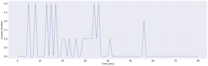
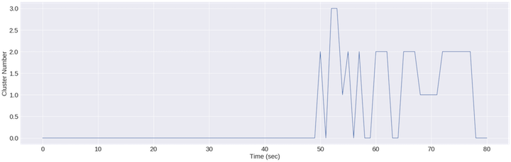
It appears that this feature isn’t perfect for clustering everything but it DOES start to carve out the eyes closed portions
Again, the above plot shows cluster assignment over time of each data point (1/256th of a second given a sampling rate of 256Hz). I’m sure my alpha signal wasn’t perfectly steady so I’m not surprised there are multiple cluster assignments between seconds 20-45. Unfortunately, this feature can’t really tell the difference between jaw clenching and head shaking, so we should look at finding that feature next.
It appears that this feature isn’t perfect for clustering everything either but it DOES start to break up the jaw clenching and head shaking.
This plot is probably exposing some of the assumptions of the kmeans algorithm, namely that each cluster ought to have the same variance. Since the variance of the magnitude feature within the jaw clenching and head shaking portion of the segment is so high, it works on minimizing variance within those clusters, while the lower variance normal and eyes closed segments look like 1 blob that doesn’t need to be broken up. The latter segment dwarfs the first 45 seconds in terms of variance.
We achieved what we set out to do: 1) exploratory data analysis on EEG data to better understand this data format, and 2) determine what features can be created and what they might be useful for.
Again, for the complete code please checkout my script here.

Leave a comment